multipath ring oscillator (MPRO)
maximum frequency
A conventional inverter-based ring oscillator consists of a single loop of an odd number of inverters. While compact, easy to design and tunable over a wide frequency range, this oscillator suffers from several limitations.
- it is not possible to increase the number of phases while maintaining the same oscillation frequency since the frequency is inversely proportional to the number of inverters in the loop. In other words, the time resolution of the oscillator is limited to one inverter delay and cannot be improved below this limit.
- the number of phases that can be obtained from this oscillator is limited to odd values. Otherwise, if an even number of inverters is used, the circuit remains in a latched state and does not oscillate.
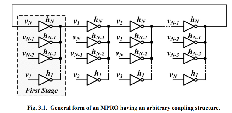
To overcome the limitations of conventional ring oscillators, multi-paths ring oscillator (MPRO) is proposed. Each phase can be driven by two or more inverters, or multi-paths instead of having each phase in oscillator driven by a single inverter, or single path.
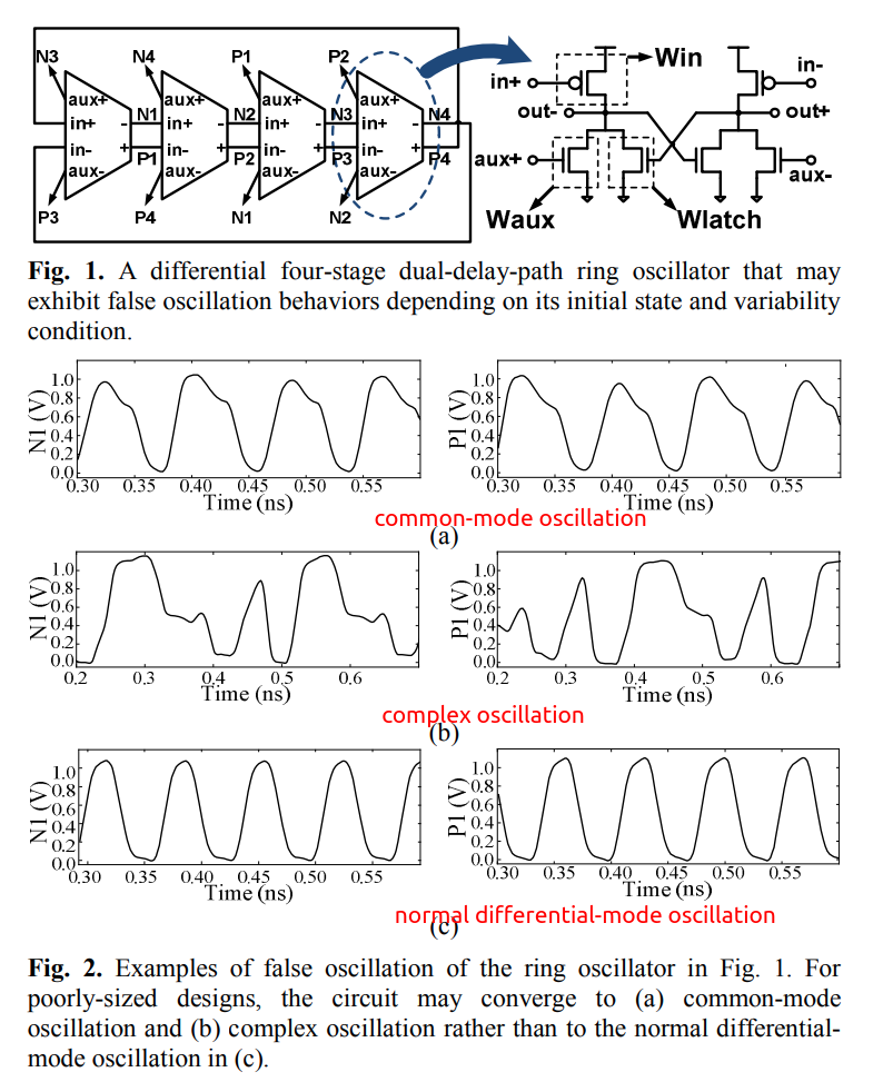
One thing that makes the MPRO design problem even more complicated is its property of having multiple possible oscillation modes. Without a clear understanding of what makes one of these modes dominant, it is very likely that a designer might end-up having an oscillator that can start-up each time in a different oscillation mode depending on the initial state of the oscillator.
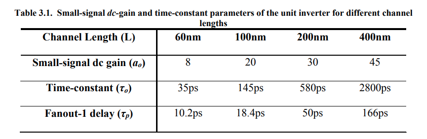
In practive, the oscillator starts first from a linear mode of operation where all the buffers are indeed acting as linear transconductors. All oscillation modes that have mode gains, \(a_n\), lower than the actual dc gain of the inverter, \(a_0\), start to grow. As the oscillation amplitude grows, the effective gain of the inverter drops due to nonlinearity. Consequently, modes with higher mode gain die out and only the mode that requires the minimum gain continues to oscillate and hence is the dominant mode.
The dominant mode is dependent only on the relative sizing vector
maximum oscillation frequency
The oscillation frequency of the dominant mode of any MPRO having any
arbitrary coupling structure and number of phases is \[
f_{n^*} = \frac {1}{2\pi}\frac {(a_0-1) \cdot \sum_{i=1}^{N}x_isin\left
( \frac {2\pi n^*(i-1)}{N} \right)}{(a_0\tau _p - \tau _o)\cdot
\sum_{i=1}^{N}-x_icos\left( \frac{2\pi n^*(i-1)}{N}+(\tau _o - \tau _p)
\right)}
\] 
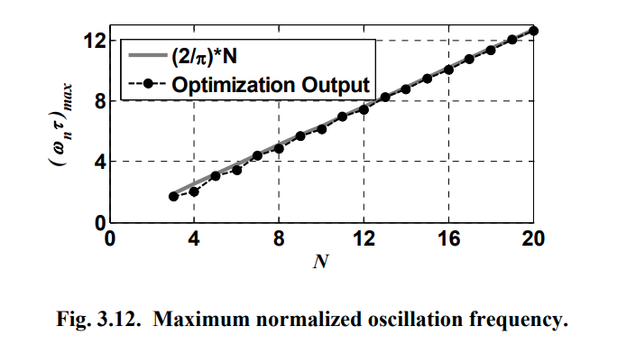
A linear increase in the maximum possible normalized oscillation frequency as the number of stages increases provided that the dc gain of the buffer sufficient to provide the required amplification
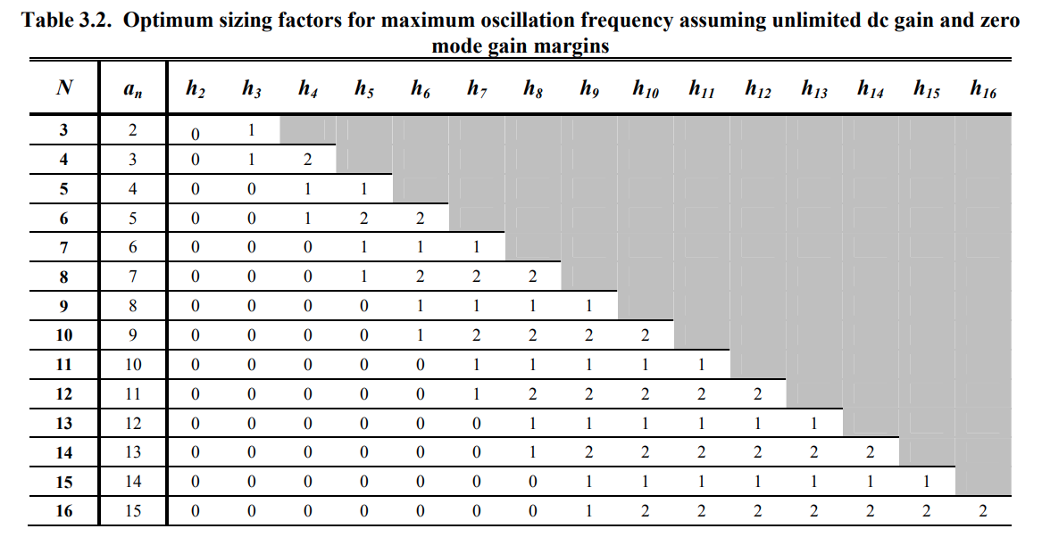
assuming unlimited dc gain and zero mode gain margins
mode stability
A common problem in MPRO design is the stability of the dominant oscillation mode. Mode stability refers to whether the MPRO always oscillates at the same mode regardless of the initial conditions of the oscillator. This problem is especially pronounced for MPROs with a large number of phases. This is due to the existence of many modes and the very small differences in the value of the mode gain of adjacent modes if the MPRO is not well designed.
In general, when the mode gain difference between two modes is small, the oscillator can operate in either one depending on initial conditions.
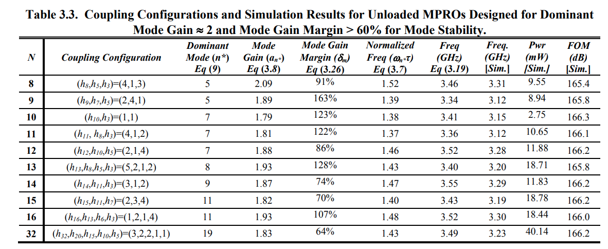
coupling configurations and simulation results
Abou-El-Sonoun, A. A. (2012). High Frequency Multiphase Clock Generation Using Multipath Oscillators and Applications. UCLA. ProQuest ID: AbouElSonoun_ucla_0031D_10684. Merritt ID: ark:/13030/m57p9288. Retrieved from https://escholarship.org/uc/item/75g8j8jt
frequency stability
A problem associated with the design of MPROs is the existence of different possible modes of oscillation. Each of these modes is characterized by a different frequency, phase shift and phase noise.
Linear delay-stage model (mode gain)
mode gain is based on the linear model, independent of process but depends on coupling structure (coupling configuration, size ratio).
The inverting buffer modeled as a linear transconductor. The input-output relationship of a single buffer scaled by \(h_i\) and driving the input capacitance of a similar buffer can be expressed as \[\begin{align} h_ig_mv_{in}(t) + h_ig_oV_{out}(t)+h_iC_g\frac {dV_{out}(t)}{dt} &= 0 \\ a_nV_{in}(t)+V_{out}(t)+\tau \frac {V_{out}(t)}{dt} &= 0 \end{align}\] where \(g_m\) is the transconductance, \(g_o\) is the output conductance, \(C_g\) is the buffer input capacitance which also acts as the load capacitance for the driving buffer, and \(a_n = \frac {g_m}{g_o}\) is the linear dc gain of the buffer, and \(\tau=\frac {C_g}{g_o}\) is a time constant.
Similarly, \(V_1\), the output of the first stage in MPRO can be expressed \[ \sum_{i=1}^{N}h_ig_mV_i(t)+\sum_{i=1}^{N}h_ig_oV_i(t)+\sum_{i=1}^{N}h_iC_g\frac {dV_it(t)}{dt} = 0 \] Defining the fractional sizing factors and the total sizing factor as \(x_i=\frac{h_i}{H}\) and \(H=\sum_{i=1}^{N}h_i\) \[ a_n\sum_{i=1}^{N}x_iV_i(t) + V_1(t)+\tau\frac {dV_i(t)}{dt} = 0 \] where \(a_n = \frac {g_m}{g_o}\) and \(\tau=\frac {C_g}{g_o}\) are same dc gain and time constant defined previously
Since the total phase shift around the loop should be multiples of \(2\pi\), the oscillation waveform at the ith node can be expressed as \[ V_i(t) = V_o \cos(\omega_nt-\Delta \varphi \cdot i) \] where \(\omega_n\) is the oscillation frequency and \(\Delta \varphi = \frac {2\pi n}{N}\), \(N\) is the number of stages in the oscillator and \(n\) can take values between \(0\) and \(N-1\)
Plug \(V_i(t)\) into differential equation, we get \[ a_n\sum_{i=1}^{N}x_i\cos(\omega_n t-\frac{2\pi n}{N}i)+\cos(\omega_n t-\frac{2\pi n}{N}) - \omega_n \tau \sin(\omega_n t-\frac{2\pi n}{N}) = 0 \] By equating the \(cos(\omega_n t)\) and \(sin(\omega_n t)\) terms of the above equation, we get expressions for the oscillation frequency of the nth mode and the minimum dc gain required for this mode to exist. we refer to this gain as the mode gain \[\begin{align} \omega_n\tau &= \frac {\sum_{i=1}^{N}x_i \cdot \sin(\frac{2\pi n}{N}(i-1))}{-\sum_{i=1}^{N}x_i \cdot \cos(\frac{2\pi n}{N}(i-1))} \\ a_n &= \frac {1}{-\sum_{i=1}^{N}x_i \cdot \cos(\frac{2\pi n}{N}(i-1))} \end{align}\] where \(a_n\) should be greater than \(0\) for a existent mode
In practice, the oscillator starts first from a linear mode of operation where all the buffers are indeed acting as linear transconductors. All oscillation modes that have mode gains \(a_n\) lower than the actual dc gain of the inverter \(a_o\) start to grow. As the oscillation amplitude grows, the effective gain of the inverter drops due to nonlinearity. Consequently, modes with higher mode gain die out and only the mode that requires the minimum gain continues to oscillate and hence is the dominant mode
A. A. Hafez and C. K. Yang, "Design and Optimization of Multipath Ring Oscillators," in IEEE Transactions on Circuits and Systems I: Regular Papers, vol. 58, no. 10, pp. 2332-2345, Oct. 2011, doi: 10.1109/TCSI.2011.2142810.
Simulation-based approach
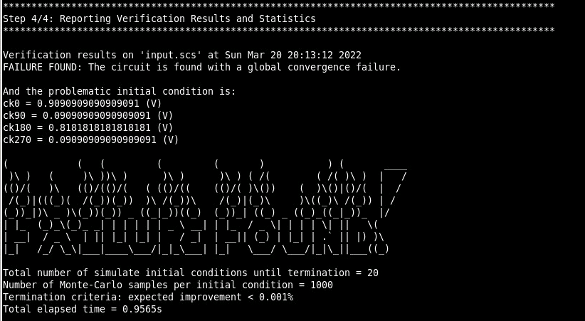
GCHECK is an automated verification tool that validate whether a ring oscillator always converges to the desired mode of operation regardless of the initial conditions and variability conditions. This is the first tool ever reported to address the global convergence failures in presence of variability. It has been shown that the tool can successfully validate a number of coupled ring oscillator circuits with various global convergence failure modes (e.g. no oscillation, false oscillation, and even chaotic oscillation) with reasonable computational costs such as running 1000-point Monte-Carlo simulations for 7~60 initial conditions (maximum 4 hours).
- The verification is performed using a predictive global optimization algorithm that looks for a problematic initial state from a discretized state space
- despite the finite number of initial state candidates considered and finite number of Monte-Carlo samples to model variability, the proposed algorithm can verify the oscillator to a prescribed confidence level
- The observation that the responses of a circuit with nearby initial conditions are strongly correlated with respect to common variability conditions enables us to explore a discretized version of the initial condition space instead of the continuous one.
- the settling time increases as the initial state gets farther away from the equilibrium state allowed us to use the settling time as a guidance metric to find a problematic initial condition.
Selecting the Next Initial Condition Candidate to Evaluate
To determine whether the algorithm should continue or terminate the search for a new maximum, the algorithm estimates the probability of finding a new initial condition with the longer settling time, based on the information obtained with the previously-evaluated initial conditions.
GCHECK EXAMPLE
1 | python gcheck_osc.py input.scs |
output log:
1 | Step 1/4: Simulating the setting-time distribution with the reference initial condition |
T. Kim, D. -G. Song, S. Youn, J. Park, H. Park and J. Kim, "Verifying start-up failures in coupled ring oscillators in presence of variability using predictive global optimization," 2013 IEEE/ACM International Conference on Computer-Aided Design (ICCAD), 2013, pp. 486-493, doi: 10.1109/ICCAD.2013.6691161.GCHECK: Global Convergence Checker for Oscillators