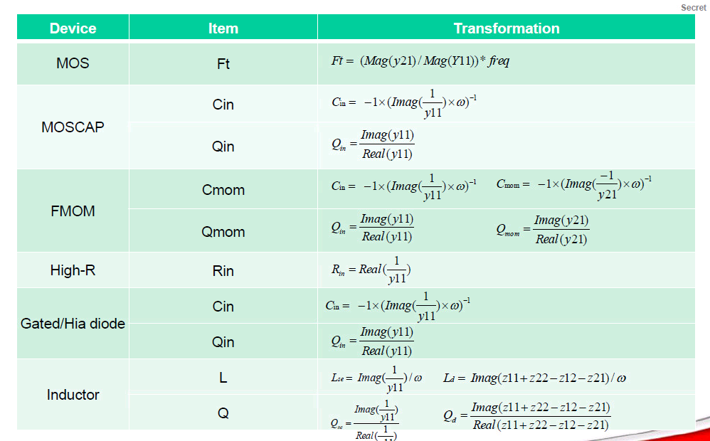
EMX & Momentum
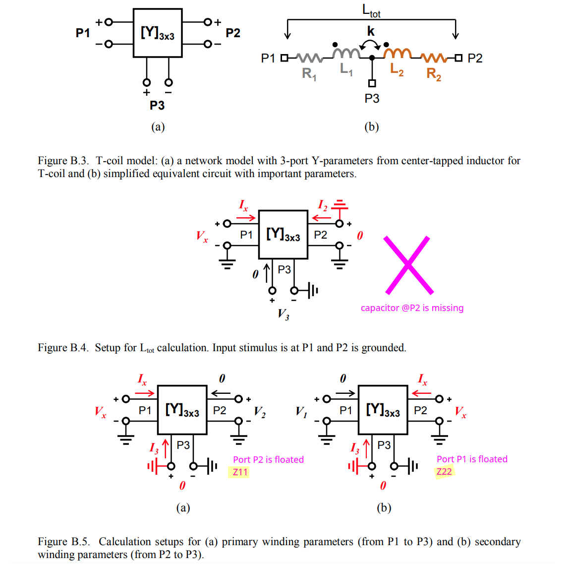
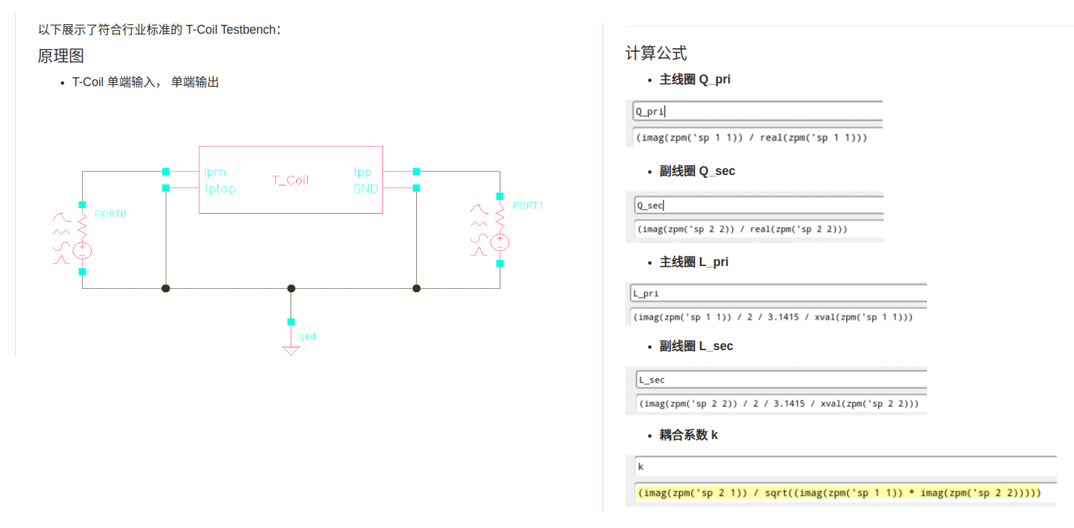
T-coil
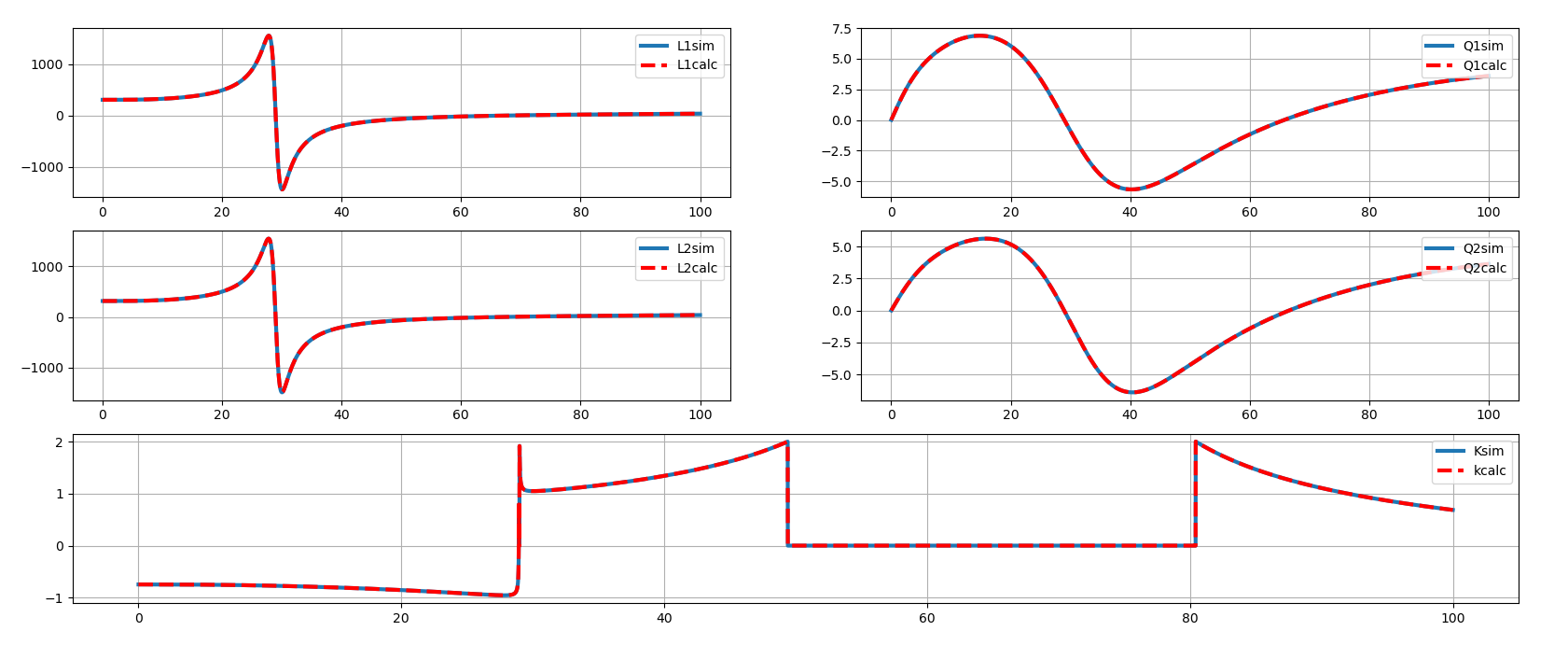
coupling factor
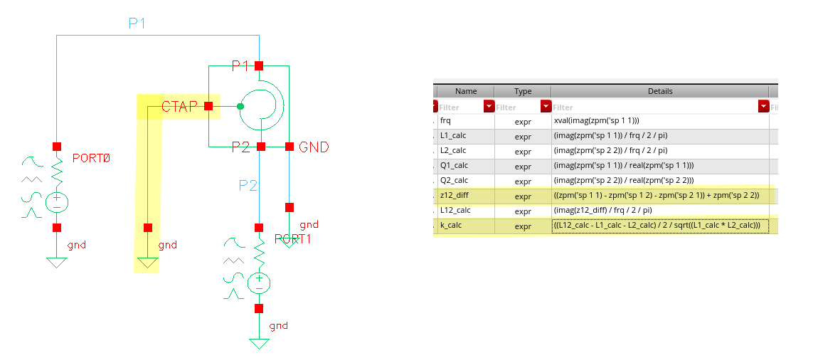
note CTAP is grounded
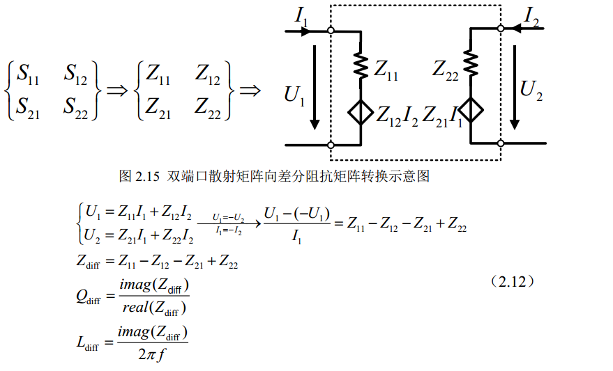
\[ L_{12} = \frac{\text{im}[Z_{diff}]}{2\pi f} \]
where \(Z_{diff} = Z_{11} - Z_{12} - Z_{21} + Z_{22}\)
Min-Sun Keel. Design of reliable and energy-efficient high-speed interface circuits. University of Illinois Urbana-Champaign, USA, 2015 [https://files.core.ac.uk/download/pdf/158312105.pdf]
1 | import numpy as np |
2
3
4
5
6
7
8
9
10
11
12
13
14
15
16
17
18
19
20
21
22
23
24
25
26
27
28
29
30
31
32
33
34
35
(lambda (l12 l1122)
(letseq ((xvec (drGetWaveformXVec l12))
(n (drVectorLength xvec))
(l12v (drGetWaveformYVec l12))
(l1122v (drGetWaveformYVec l1122))
(resultv (drCreateVec 'double n)))
(do ((i 0 i+1))
((i >= n))
(letseq ((l12i (drGetElem l12v i))
(l1122i (drGetElem l1122v i))
(kk (if (l1122i > 0.0)
l12i/(sqrt l1122i)
0.0))
(k (if ((abs kk) < 2.0) kk 0.0)))
(drSetElem resultv i k)))
(drCreateWaveform xvec resultv)))))
(EMX_plot_aux bgui wid what 3
'("Inductance" "Q" "k")
'("Henry" "" "")
(lambda (ys)
(letseq ((zs (reduce ys))
(z11 (nth 0 zs))
(z12 (nth 1 zs))
(z22 (nth 2 zs))
(pi 3.14159265358979)
(f (xval z11))
(l11 (imag z11)/(2*pi*f))
(q11 (imag z11)/(real z11))
(l12 (imag z12)/(2*pi*f))
(l22 (imag z22)/(2*pi*f))
(q22 (imag z22)/(real z22))
(k (get_k l12 l11*l22)))
`((,l11 ,l22) (,q11 ,q22) (,k))))
'(("L1" "L2") ("Q1" "Q2") ("k")))))
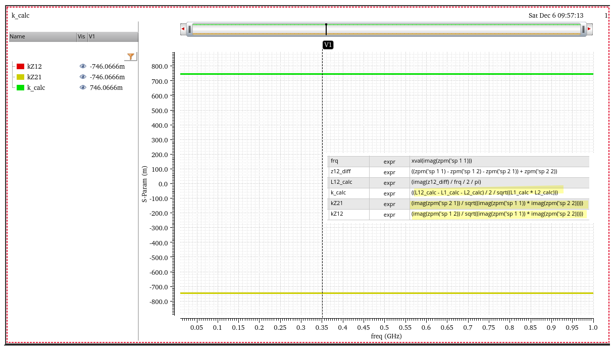
\[
k = \frac{L_{tot}-L_1-L_2}{2M} = \frac{\text{im}[Z_{diff}]/2\pi f -
\text{im}[Z_{11}]/2\pi f-\text{im}[Z_{22}]/2\pi
f}{2\sqrt{\text{im}[Z_{11}]/2\pi f\times \text{im}[Z_{22}]/2\pi f}} =
\frac{- \text{im}[Z_{12}] -
\text{im}[Z_{21}]}{2\sqrt{\text{im}[Z_{11}]\times \text{im}[Z_{22}]}}
\] if \(\text{im}[Z_{12}] =
\text{im}[Z_{21}]\), then \[
\color{red}k =- \frac{\text{im}[Z_{21}]}{\sqrt{\text{im}[Z_{11}]\times
\text{im}[Z_{22}]}}
\] 
\(C_B\) from Nport
Chapter 4.5. High Frequency Passive Devices [https://www.cambridge.org/il/files/7713/6698/2369/HFIC_chapter_4_passives.pdf]
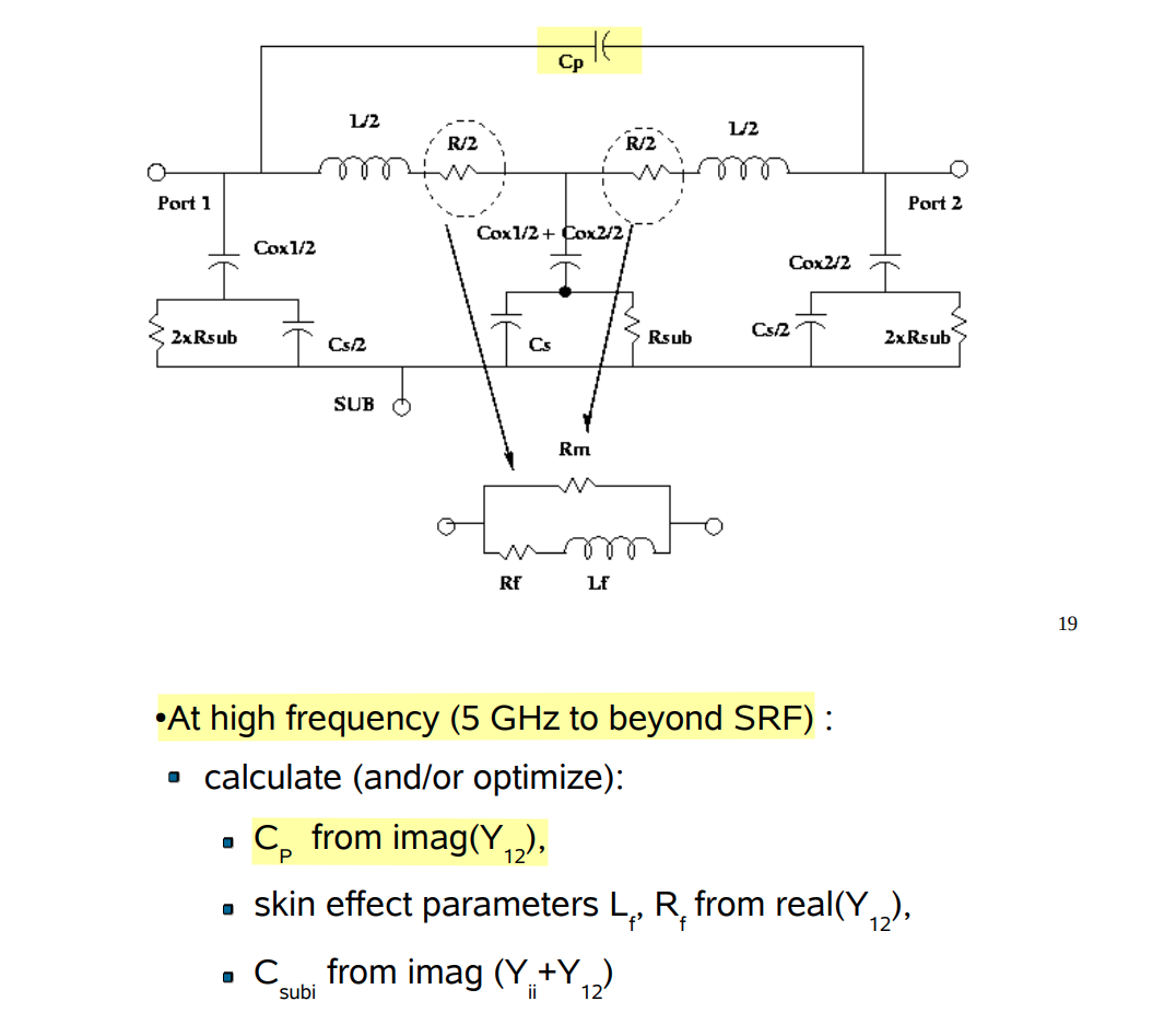
Min-Sun Keel. Design of reliable and energy-efficient high-speed interface circuits. University of Illinois Urbana-Champaign, USA, 2015 [https://files.core.ac.uk/download/pdf/158312105.pdf]
Measuring Self Resonant Frequency [https://www.coilcraft.com/getmedia/8ef1bd18-d092-40e8-a3c8-929bec6adfc9/doc363_measuringsrf.pdf?srsltid=AfmBOoqdBJ_CTB-N_wOVp2_7zIDXPEwOYLm7S4RLuws1CEcEWZUijblK]
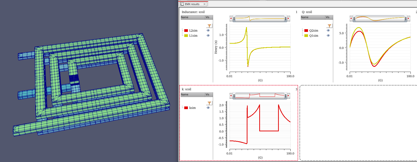
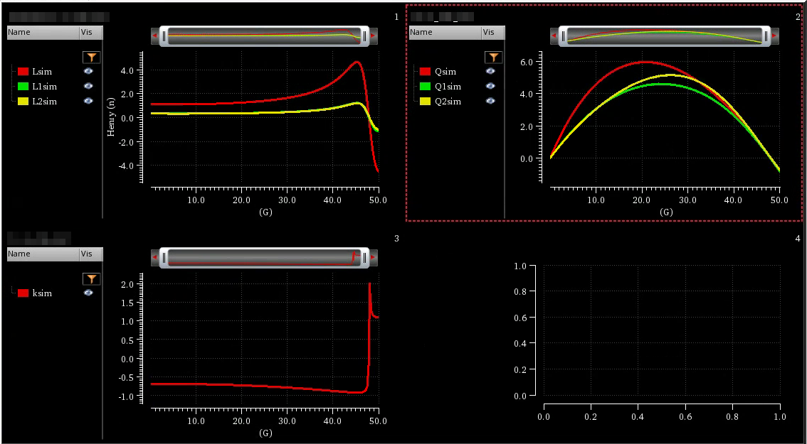
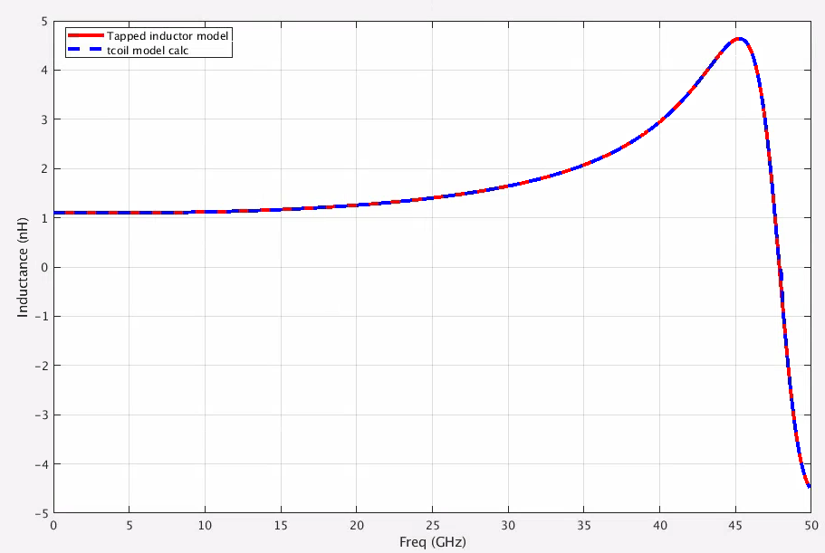
T-coil vs tapped inductor
tcoil and tapped inductor share same EM simulation result, and use modelgen with different model formula.
The relationship is \[ L_{\text{sim}} = L1_{\text{sim}}+L2_{\text{sim}}+2\times k_{\text{sim}} \times \sqrt{L1_{\text{sim}}\cdot L2_{\text{sim}}} \] where \(L1_{\text{sim}}\), \(L2_{\text{sim}}\) and \(k_{\text{sim}}\) come from tcoil model result, \(L_{\text{sim}}\) comes from tapped inductor model result
\(k_{\text{sim}}\) in EMX have assumption, induce current from P1 and P2 Given Dot Convention:
Same direction : k > 0
Opposite direction : k < 0
So, the \(k_{\text{sim}}\) is negative if routing coil in same direction
1 | % EMX - shield tcoil model |
Transformer
J. R. Long, "On-chip transformer design and application to RF and mm-wave front-ends," 2017 IEEE Custom Integrated Circuits Conference (CICC), Austin, TX, USA, 2017 [pdf]
A. Bevilacqua, "Tutorial: Fundamentals of Integrated Transformers: from Principles to Applications," 2020 IEEE International Solid-State Circuits Conference - (ISSCC), San Francisco, CA, USA, 2020 [pdf]
—, "Fundamentals of Integrated Transformers: From Principles to Applications," in IEEE Solid-State Circuits Magazine, vol. 12, no. 4, pp. 86-100, Fall 2020

[https://wiki.icprophet.com/doku.php?id=wiki#%E5%8F%98%E5%8E%8B%E5%99%A8]
| 变压器差分输入、差分输出 |  |
|---|---|
| 变压器单端输入、差分输出 |  |
| 变压器差分输入、单端输出 |  |
| 变压器单端输入、单端输出 |  |
the formula is same with T-coil's
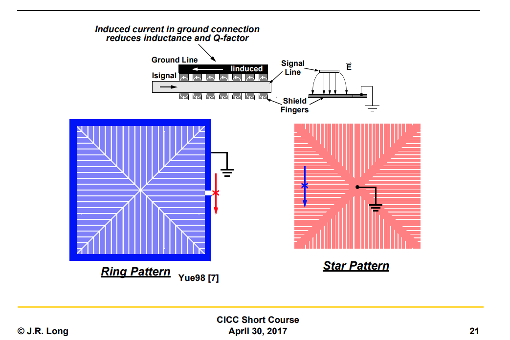
PGS (Patterned ground Shields)
Ring Pattern, Star Pattern
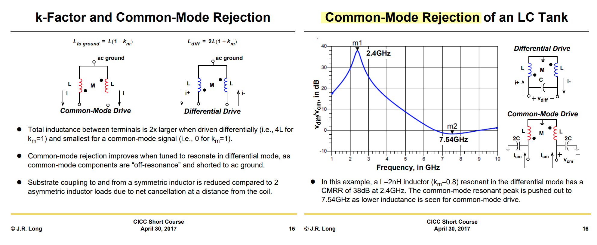
Common-Mode Rejection
TODO 📅
Transmission Zero
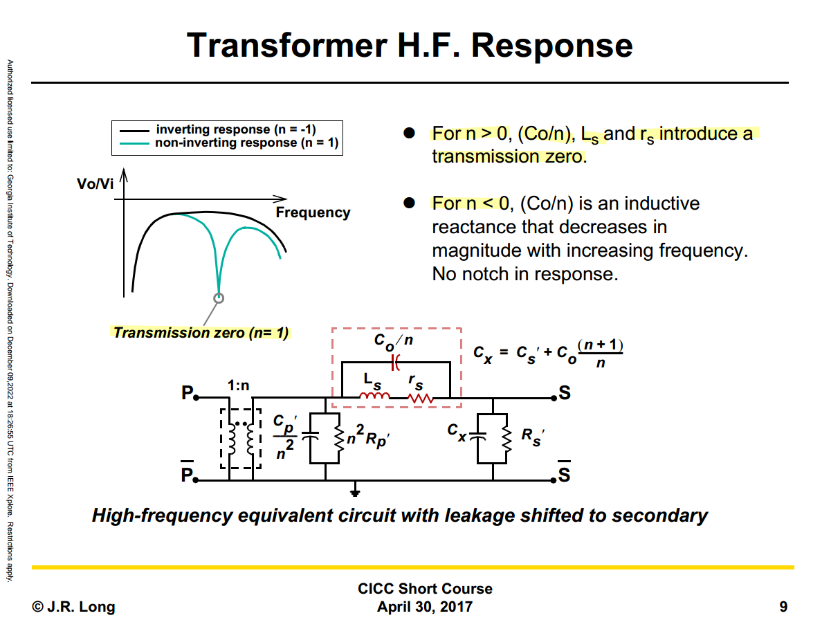
like shunt-peaking, the impedance of \(C_o/n\), \(L_s\), \(r_s\) have resonant peak at resonant frequency, which block signal transmission to S
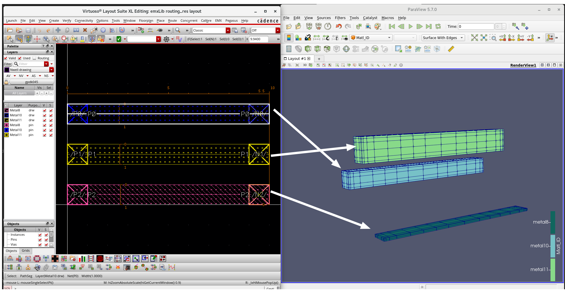
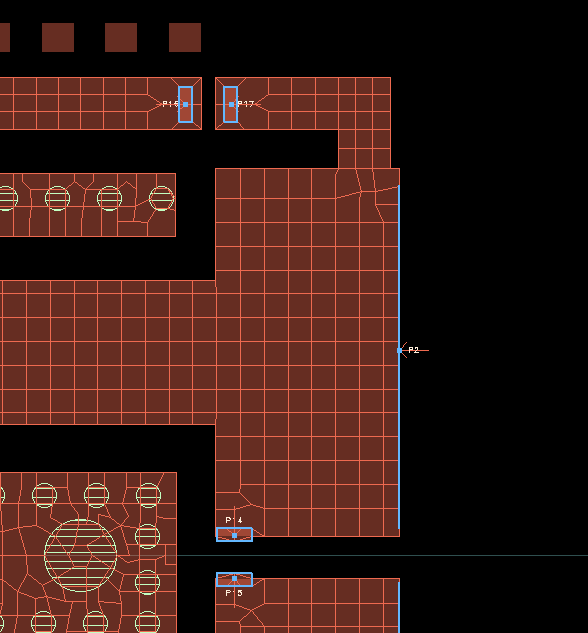
EMX ports
plain labels
- pin layer
- uncheck Cadence pins in Advanced options
rectangle pins
- drawing layer rectangle pin and specify Access Direction as intended
- check Cadence pins in Advanced options
The rectangle pins are always selected as driven port while there are only rectangle pin whether Cadence pins checked or not.
check ports used for simulation
use GDS view - EMX
EMX Synthesis Kits
Synthesis is a capability of the EMX Pcell library and uses scalable model data pre-generated by Continuum for a specific process and metal scheme combination.
Synthesis is supported by the Pcells that are suffixed _scalable, and these Pcells have the additional fields and buttons needed for synthesis.
port order (signals)
emxform.ils
| type | Port order |
|---|---|
| inductor | P1 P2 |
| shield inductor | P1 P2 SHIELD |
| tapped inductor | P1 P2 CT |
| tapped shield inductor | P1 P2 CT SHIELD |
| mom/mim capacitor | P1 P2 |
| tcoil | P1 P2 TAP |
| shield tcoil | P1 P2 TAP SHIELD |
| tline | P1 P2 |
| differential tline | P1 P2 P3 P4 |
EMX device info
| name | menu_selection (split with _ ) | num_ports | modelgen_type | generic_model_type | plot_fn |
|---|---|---|---|---|---|
| Single-ended inductor | inductor_no tap_no shield_single-ended | 2 | inductor | inductor | EMX_plot_se_ind |
| Differential inductor | inductor_no tap_no shield_differential | 2 | inductor | inductor | EMX_plot_diff_ind |
| Single-ended shield inductor | inductor_no tap_with shield_single-ended | 3 | shield_inductor | shield_inductor | EMX_plot_se_ind |
| Differential shield inductor | inductor_no tap_with shield_differential | 3 | shield_inductor | shield_inductor | EMX_plot_diff_ind |
| Tapped inductor (diff mode only) | inductor_with tap_no shield_differential mode only | 3 | center_tapped_inductor | tapped_inductor | EMX_plot_ct_ind |
| Tapped inductor (common mode too) | inductor_with tap_no shield_also fit common mode | 3 | center_tapped_inductor_common_mode | tapped_inductor | EMX_plot_ct_ind |
| Tapped shield inductor (diff only) | inductor_with tap_with shield_differential mode only | 4 | center_tapped_well_inductor_common_mode | tapped_shield_inductor | EMX_plot_ct_ind |
| Single-ended cap (symm) | capacitor_symmetric single-ended | 2 | complex_mom_capacitor | mom_capacitor | EMX_plot_se_cap |
| Differential cap (symm) | capacitor_symmetric differential | 2 | complex_mom_capacitor | mom_capacitor | EMX_plot_diff_cap |
| Single-ended cap (asymm) | capacitor_asymmetric single-ended | 2 | complex_asymmetric_mom_capacitor | mom_capacitor | EMX_plot_se_cap |
| Differential cap (asymm) | capacitor_asymmetric differential | 2 | complex_asymmetric_mom_capacitor | mom_capacitor | EMX_plot_diff_cap |
| MiM capacitor | capacitor_MiM | 2 | mim_capacitor | mim_capacitor | EMX_plot_se_cap |
| Tcoil (simple model) | tcoil_simple model | 3 | tcoil | tcoil | EMX_plot_tcoil |
| Tcoil (complex model) | tcoil_complex model | 3 | complex_tcoil | complex_tcoil | EMX_plot_tcoil |
| Shield tcoil | tcoil_with shield | 4 | shield_complex_tcoil | shield_tcoil | EMX_plot_shield_tcoil |
| Transmission line | transmission line_single | 2 | xline | xline | EMX_plot_xline |
| Diff transmission line | transmission line_coupled (differential) | 4 | coupled_xline | diff_xline | EMX_plot_diff_xline |
EMX plot function
EMX's formulation is defined in
EMX import this file at Virtuoso startup, you have to relaunch Virtuoso if you change this file
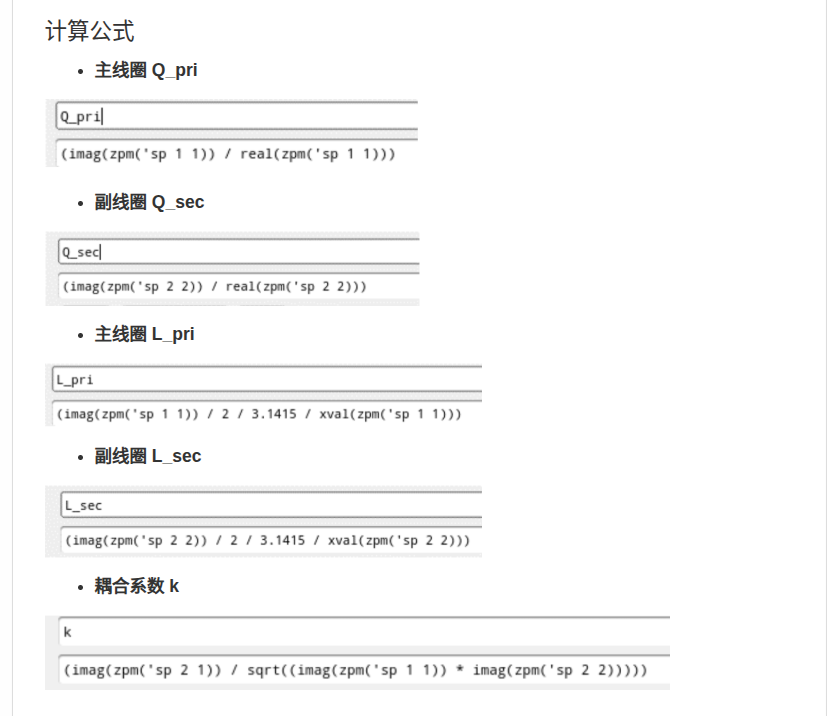
Single-ended inductor
Both with and without shield apply
- port-1 impedance when port-2 short
\[ Z_1 = \frac{1}{Y_{11}} \]
- port-2 impedance when port-1 short
\[ Z_2 = \frac{1}{Y_{22}} \] Then \[\begin{align} L1 &= \frac{Im(Z_1)}{2\pi f} \\ Q1 &= \frac{Im(Z_1)}{Re(Z_1)} \\ L2 &= \frac{Im(Z_2)}{2\pi f} \\ Q2 &= \frac{Im(Z_2)}{Re(Z_2)} \end{align}\]
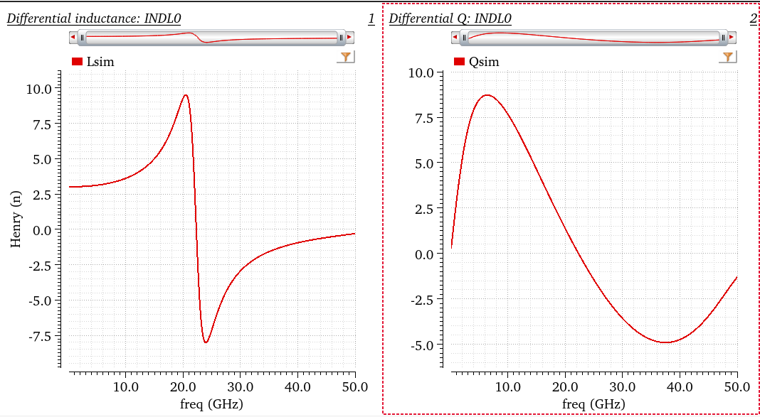
EMX only plot L1 and Q1
Differential inductor
Both with and without shield apply
\[\begin{align} L_{diff} &= \frac{Im(Z_{diff})}{2\pi f} \\ Q_{diff} &= \frac{Im(Z_{diff})}{Re(Z_{diff})} \end{align}\]
Center-tapped inductor
\[ Y = \begin{bmatrix} Y_{11} & Y_{12} & Y_{13}\\ Y_{21} & Y_{22} & Y_{23}\\ Y_{31} & Y_{32} & Y_{33} \end{bmatrix} \]
where port order is P1 P2 CT.
1 | (define (EMX_plot_ct_ind bgui wid what) |
Assume CT i.e. port 3 in S-parameter is grounded,
(z (EMX_differential (nth 0 ys) (nth 1 ys) (nth 3 ys) (nth 4 ys)))
obtain differential impedance with \(Y_{11}\), \(Y_{12}\), \(Y_{21}\) and \(Y_{22}\). \[
Y =
\begin{bmatrix}
Y_{11} & Y_{12}\\
Y_{21} & Y_{22}
\end{bmatrix}
\] Finally, differential inductance and Q are obtained, shown as
below
\[\begin{align} L_{diff} &= \frac{Im(Z_{diff})}{2\pi f} \\ Q_{diff} &= \frac{Im(Z_{diff})}{Re(Z_{diff})} \end{align}\]
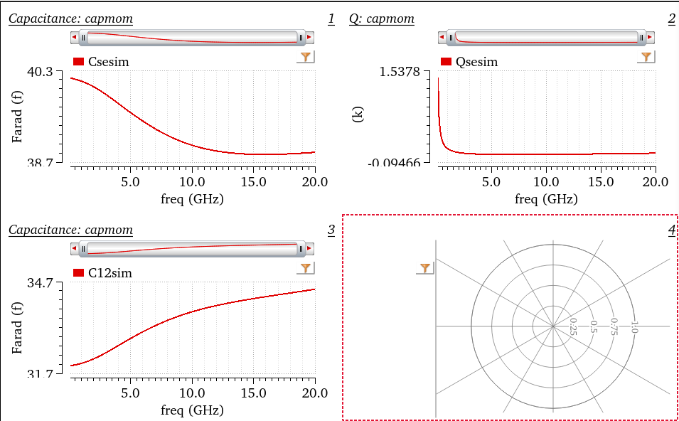
Single-ended cap
1 | (define (EMX_plot_se_cap bgui wid what) |
We define Port-1 impedance \(Z_1\), Port-2 impedance \(Z_2\)
\[\begin{align} Z_1 &= \frac {1}{Y_{11}}\\ Z_2 &= \frac {1}{Y_{22}} \end{align}\]
Caution above \(\color{red}z_1 \neq Z_{11}\), but \(z_1=\frac{1}{Y_{11}}\)
Then single-ended cap and Q \[\begin{align} C_1 &= -\frac{1/Im(Z_1)}{2\pi f} \\ Q_1 &= -\frac{Im(Z_1)}{Re(Z_1)} \\ C_2 &= -\frac{1/Im(Z_2)}{2\pi f} \\ Q_2 &= -\frac{Im(Z_2)}{Re(Z_2)} \\ C_{12} &= -\frac{Im(Y_{12})}{2\pi f}\\ Q_{12} &= \frac{Im(Y_{12})}{Re(Y_{12})} \end{align}\]
- Series equivalent model is used in \(C_1\), \(Q_1\), \(C_2\) and \(Q_2\)
- \(Z_1 = R + \frac{1}{sC_1}\) and \(Z_2 = R + \frac{1}{sC_2}\)
- Parallel model is used in \(C_{12}\) and \(Q_{12}\)
- \(Y_{12} = \frac{1}{R} + sC_{12}\)
EMX plot \(C_{se}\), \(Q_{se}\) and \(C_{12}\), i.e. \(C_1\), \(Q_1\) and \(C_{12}\)
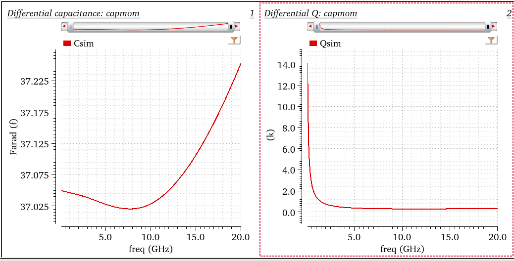
Differential cap
1 | (define (EMX_plot_diff_cap bgui wid what) |
First obtain differential impedance, \(Z_{diff}\) then apply series equivalent model \[\begin{align} C_{diff} &= -\frac{1/Im(Z_{diff})}{2\pi f} \\ Q_{diff} &= -\frac{Im(Z_{diff})}{Re(Z_{diff})} \end{align}\]
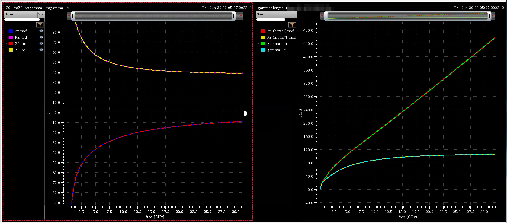
Tline
Open circuit impedance \(Z_o\), short circuit impedance \(Z_s\) and characteristic impedance \(Z_0\)
\[\begin{align} Z_o &= Z_{11}\\ Z_s &= \frac{1}{Y_{11}}\\ Z_0 &= \sqrt{Z_o*Z_s} \end{align}\]
propagation constant is given as
\[\gamma \cdot l = \frac{1}{2}\log\left( \frac{Z_0+Z_s}{Z_0-Z_s} \right)\]
\(Z_s\) depends on the length of tline [Google AI Mode]
The relationship between these parameter and geometry of the transmission line \[\begin{align} Z_0 &= \sqrt{\frac{R+j\omega L}{G+j\omega C}} \\ \gamma &= \sqrt{(G+j\omega C)(R+j\omega L)} \end{align}\] EMX plot the real and imaginary part of \(Z_0\), \(\alpha\) and \(\beta\) of \(\gamma\)
Note EMX plot the absolute value of \(\alpha\) and \(\beta\)
EMX autoplot
using AC simulation, and inductor's parallel model or series model
That is to say: both
sp(network parameter) andac(impedance) can be used to plot inductance, Q value.usually EMX choose
acmethod
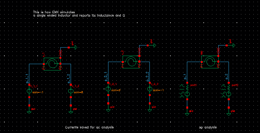
left 2 figures are used for AC simulation, \(Y_{nn}\) can be obtained conveniently
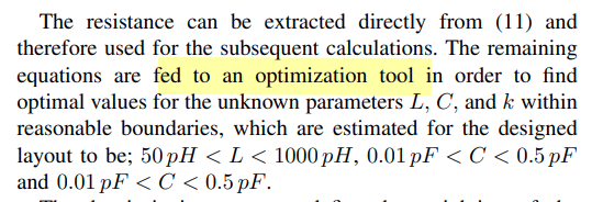
Model parameter extraction
Chapter 4.5. High Frequency Passive Devices [https://www.cambridge.org/il/files/7713/6698/2369/HFIC_chapter_4_passives.pdf]
for single-end capicator \[\begin{align} Q_1 &= -\frac{Im(Z_1)}{Re(Z_1)} \\ &= -\frac{Im(1/Y_{11})}{Re(1/Y_{11})} \\ &= -\frac{Im(Y_{11}^*)/|Y_{11}|^2}{Re(Y_{11}^*)/|Y_{11}|^2} \\ &= \frac{Im(Y_{11})}{Re(Y_{11})} \end{align}\]
So, the EMX model and foundary model is consistent.
O. Hanay, J. Hulsman and R. Negra, "Three-Port S-Parameter based characterization of integrated bridged-T-Coils," 2019 12th German Microwave Conference (GeMiC), Stuttgart, Germany, 2019, pp. 268-271 [https://sci-hub.se/10.23919/GEMIC.2019.8698123]
pad & bump
EMX process file contain M0 up to RDL-AP
PM, CB2_FC, UBM is in the chip package
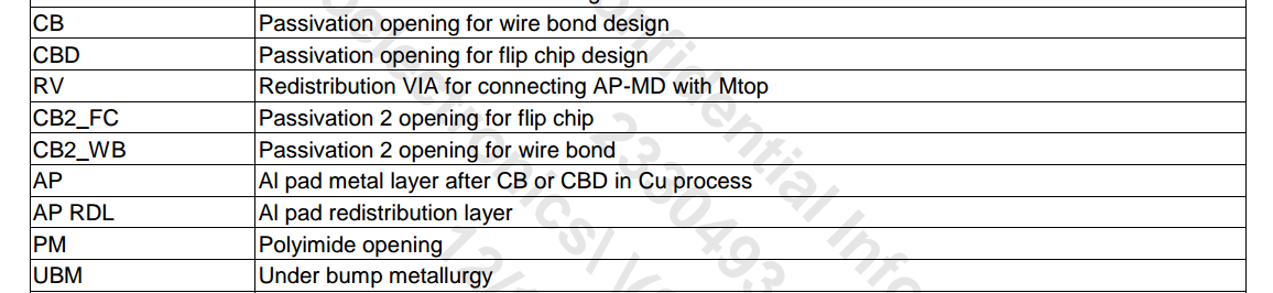
PEX extract up to RDL-AP as expected
DC model
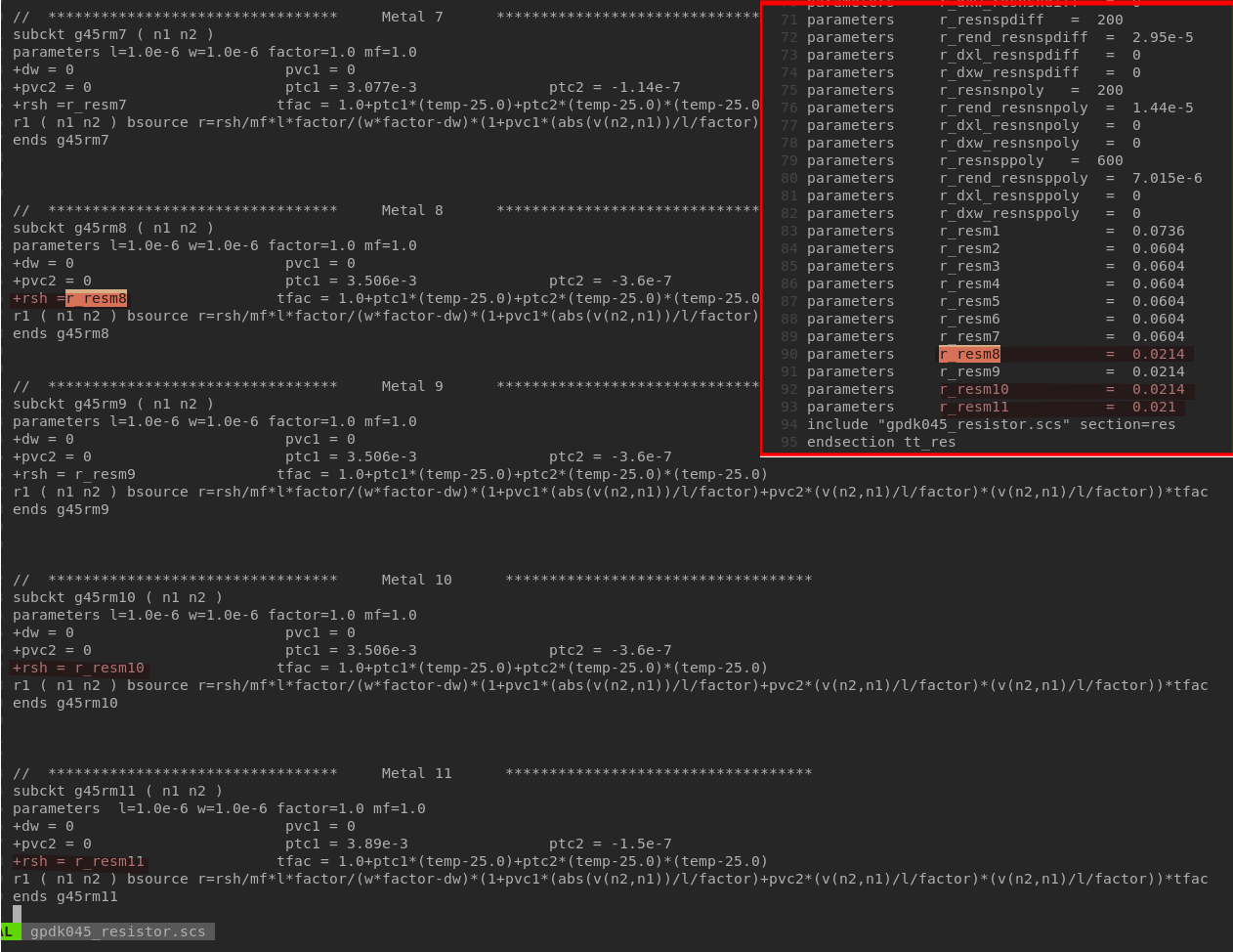
quick find routing resistance
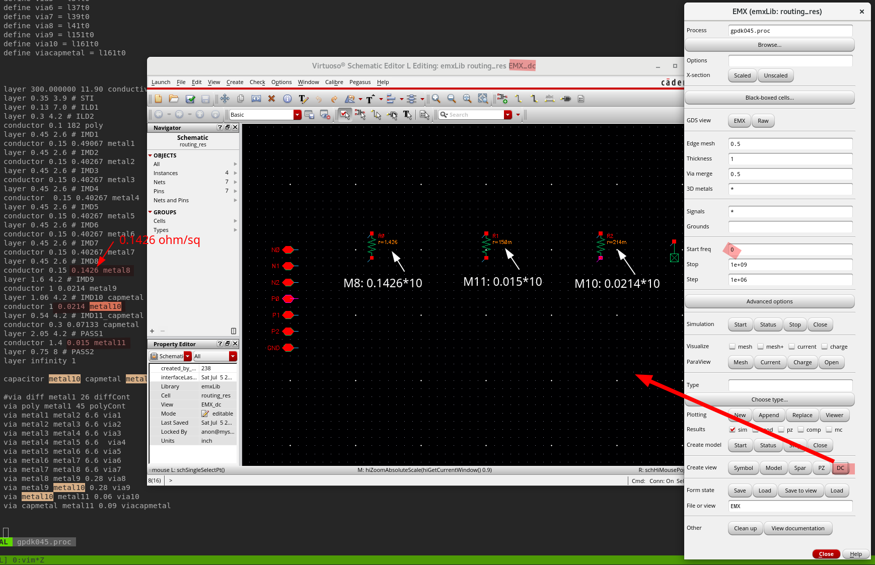
GPDK045 metal resistor model is not consistent with its process file on sheet resistance
Mixed-Mode Z/Y-Parameters
Mixed-Mode Y/Z-Parameters [http://zeptoblog.com/2024/03/09/mixed-mode-yz-parameters.html]
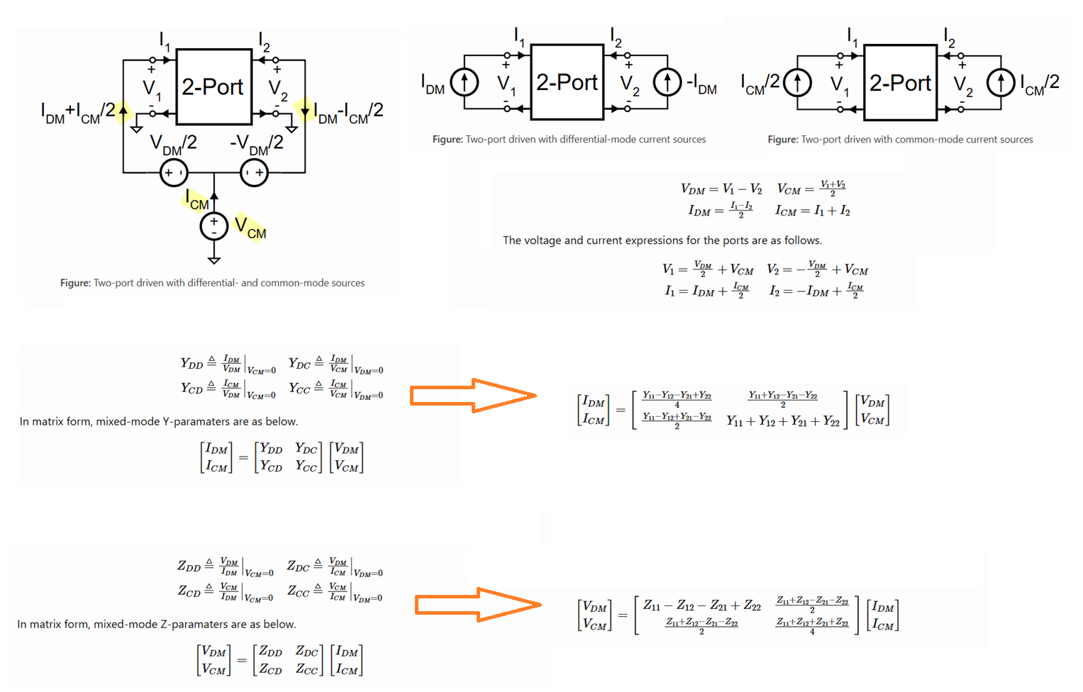
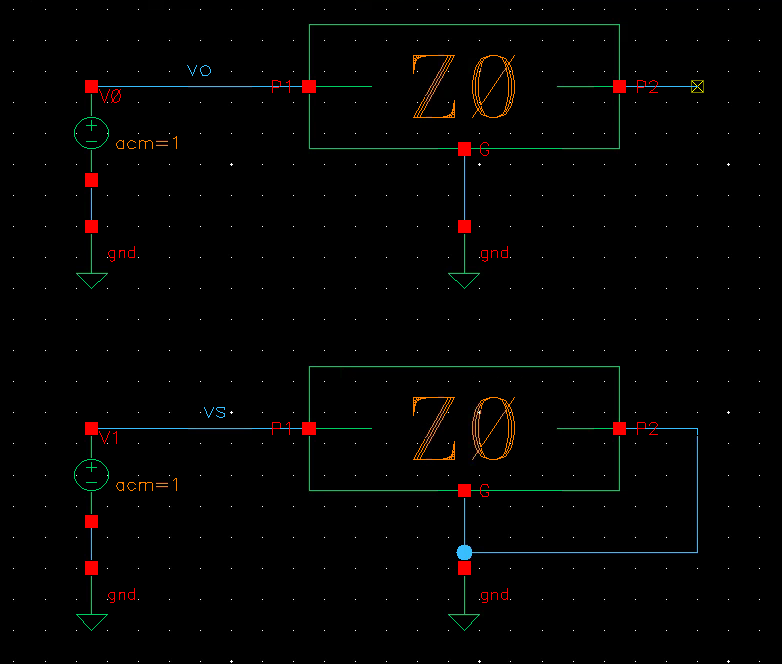
DE & SE excitation
Min-Sun Keel. Design of reliable and energy-efficient high-speed interface circuits. University of Illinois Urbana-Champaign, USA, 2015 [https://files.core.ac.uk/download/pdf/158312105.pdf]
differential impedance
Y parameters to Z parameters
\[\begin{align} |Y| &= Y_{11}*Y_{22} - Y_{12}*Y_{22} \\ \begin{bmatrix} Z_{11} & Z_{12}\\ Z_{21} & Z_{22} \end{bmatrix} &= \begin{bmatrix} \frac{Y_{22}}{|Y|} & \frac{-Y_{12}}{|Y|}\\ \frac{-Y_{21}}{|Y|} & \frac{Y_{11}}{|Y|} \end{bmatrix} \end{align}\]
Then differential impedance is \[ Z_{diff} = Z_{11} - Z_{12} - Z_{21} + Z_{22} \]
1 | (define (EMX_differential y11 y12 y21 y22) |
similarly, Z parameters to Y parameters \[ \begin{bmatrix} Y_{11} & Y_{12}\\ Y_{21} & Y_{22} \end{bmatrix} = \begin{bmatrix} \frac{Z_{22}}{|Z|} & \frac{-Z_{12}}{|Z|}\\ \frac{-Z_{21}}{|Z|} & \frac{Z_{11}}{|Z|} \end{bmatrix} \] where \[ |Z| = Z_{11}Z_{22} - Z_{12}Z_{21} \]
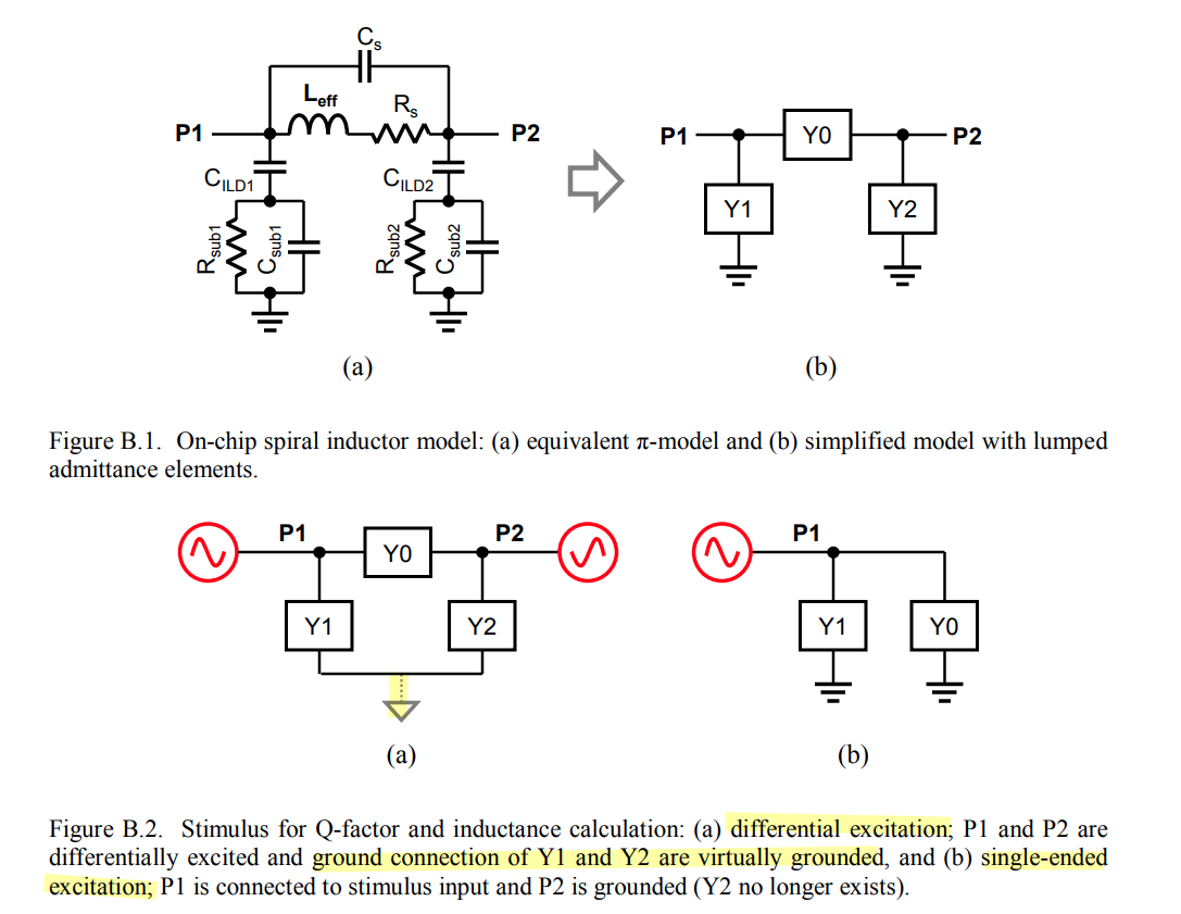
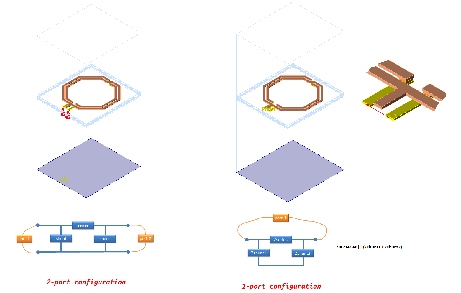
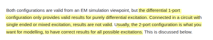
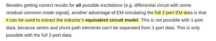
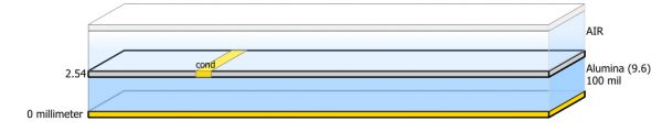
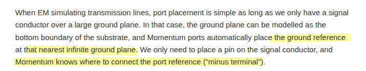
Inductor EM simulation: 1-port or 2-port? [https://muehlhaus.com/support/ads-application-notes/inductor-em-ports]
Ports & Ground Reference
The ground pin confusion in EM transmission line models [https://muehlhaus.com/support/ads-application-notes/em_line_ground]
Momentum port: global ground or differential? [https://muehlhaus.com/support/ads-application-notes/momentum-port-global-ground-or-differential]
Effect of ground cutout size on RFIC inductor performance [https://muehlhaus.com/support/rfic-em-appnotes/inductor-ground-cutout]
dummy metal fill
60 GHz on-chip balun transformer: effect of dummy metal fill [https://muehlhaus.com/support/rfic-em-appnotes/60-ghz-balun-filler-effect]
TODO 📅
Edge/Area pins in Momentum
Edge/Area pins in Momentum EM simulation [https://muehlhaus.com/support/ads-application-notes/edge-area-pins]
For accurate results from EM, the current in the model needs to flow in the physically correct way, similar to the hardware. With edge/area pins, we can help Momentum to create the physically correct current flow in complex port configurations.
Edge port with user defined location and size
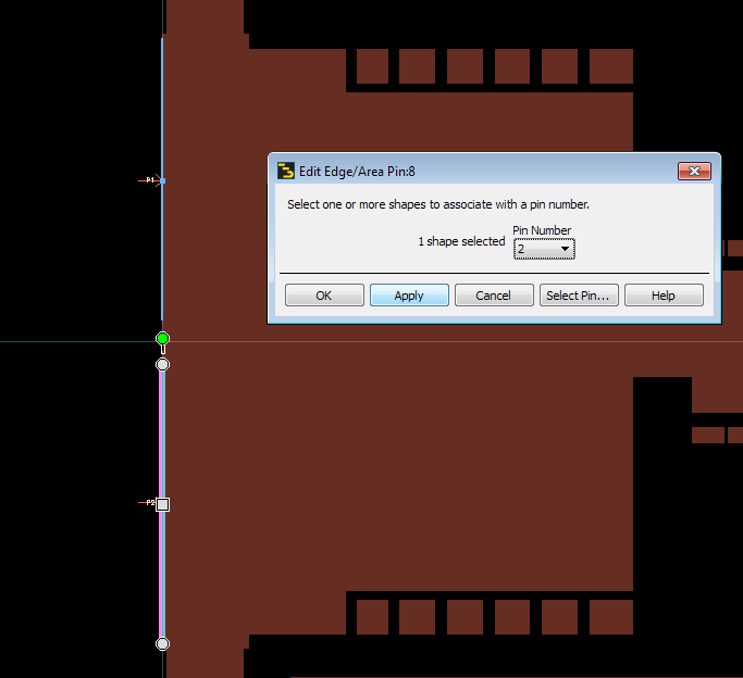
Area pins with user defined location and size
If we manually control the area pin size, Momentum will equally distribute the injected current across that area
same Pin names in EMX
It remains shrouded in myth
Setup Tricks
Process file*
Process file encryption mostly for advanced nodes, like TSMC 16nm Finfet, whose process file is encrypted.
- Use
--key=EMXkeyin the EMX Advanced options
GDSviewer has two options
- EMX: shows the final gds sent to EMX for simulation after it has been processed by EMX
- Raw: shows the raw gds
If there are port name with the
#sign, it means EMX sees a port but it is not in the signal list.
EMX Accuracy
Edge mesh: controls layout discretization in the X-Y plane
- For MoM capacitors, use the edge mesh to be the same as the width of the finger (for example, 0.1um).
Thickness: controls layout discretization in the Z dimension
3D metals: skips all 2D assumptions about conductors and their currents and charges
- If you set
3D metalsto*then all metals are treated as 3D- For Inductor type structures, only thick metal needs 3D.
- For MoM, all layers are needed.
- If you set
Ports entered in Grounds will cause these nets to be
grounded; these ports will not show up in the S-parameter result.
Setup Temperature
- EMX:
--temperature=100
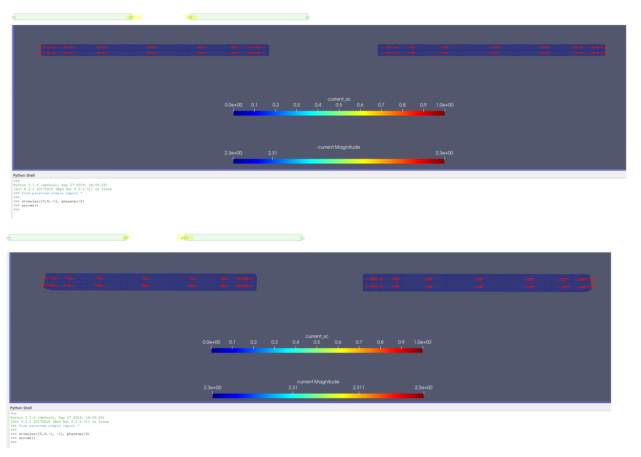
ParaView
- If check ParaView related options when ParaView is not setup properly, EMX simulation stop at Creating mesh... without waring or errors (version 6.2).
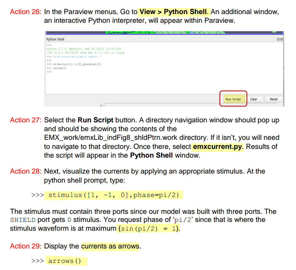
Paraview & stimulus
LVS check
LVS issue for circuits with customized devices
auCdl: Analog and Microwave CDL, is a netlister used for creating CDL netlist for analog circuits
auLVS: Analog and Microwave LVS, is used for analog circuit LVS
reference
Tips on Specifying Ports in EMX
Using 'Cadence pins' as ports with access direction in EMX simulations
EMX miscellaneous features [https://picture.iczhiku.com/resource/eetop/WyIFKleSLTRIuvCb.pdf]
Cadence Rapid Adoption Kit (RAK). Analysis of a Figure-Eight Inductor with EMX