Laplace Transform and z-Transform in System Analysis
The Laplace transform converts integro-differential equations into algebraic equations - continuous-time systems
The z-transforms changes difference equations into algebraic equations - discrete-time systems
FIR Equalization
Frequency Response
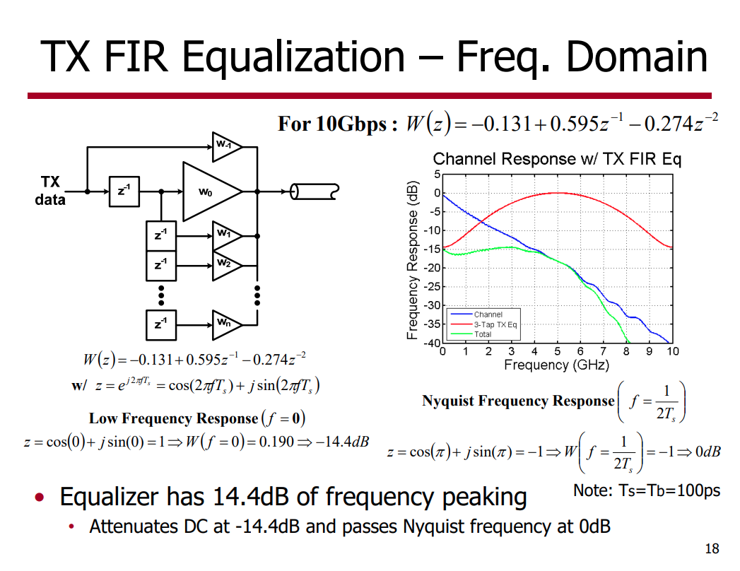 \[
z = e^{j\omega T_s}
\]
\[
z = e^{j\omega T_s}
\]
Unit impulse
filter coefficients are [-0.131, 0.595, -0.274] and sampling period is 100ps
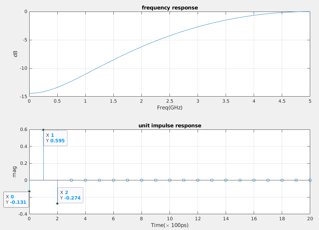
1 | %% Frequency response |
impulse:For discrete-time systems, the impulse response is the response to a unit area pulse of length
Tsand height1/Ts, whereTsis the sample time of the system. (This pulse approaches \(\delta(t)\) asTsapproaches zero.)Scale output:
Multiply
impulseoutput with sample periodTsin order to correct1/Tsheight ofimpulsefunction.
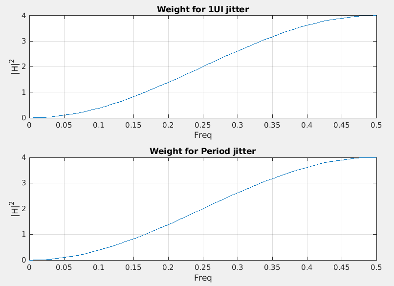
PSD transformation
If we have power spectrum or power spectrum density of both edge's absolute jitter (\(x(n)\)) , \(P_{\text{xx}}\)
Then 1UI jitter is \(x_{\text{1UI}}(n)=x(n)-x(n-1)\), and Period jitter is \(x_{\text{Period}}(n)=x(n)-x(n-2)\), which can be modeled as FIR filter, \(H(\omega) = 1-z^{-k}\), i.e. \(k=1\) for 1UI jitter and \(k=2\) Period jitter \[\begin{align} P_{\text{xx}}'(\omega) &= P_{\text{xx}}(\omega) \cdot \left| 1-z^{-k} \right|^2 \\ &= P_{\text{xx}}(\omega) \cdot \left| 1-(e^{j\omega T_s})^{-k} \right|^2 \\ &= P_{\text{xx}}(\omega) \cdot \left| 1-e^{-j\omega T_s k} \right|^2 \end{align}\]
1 | clear all |
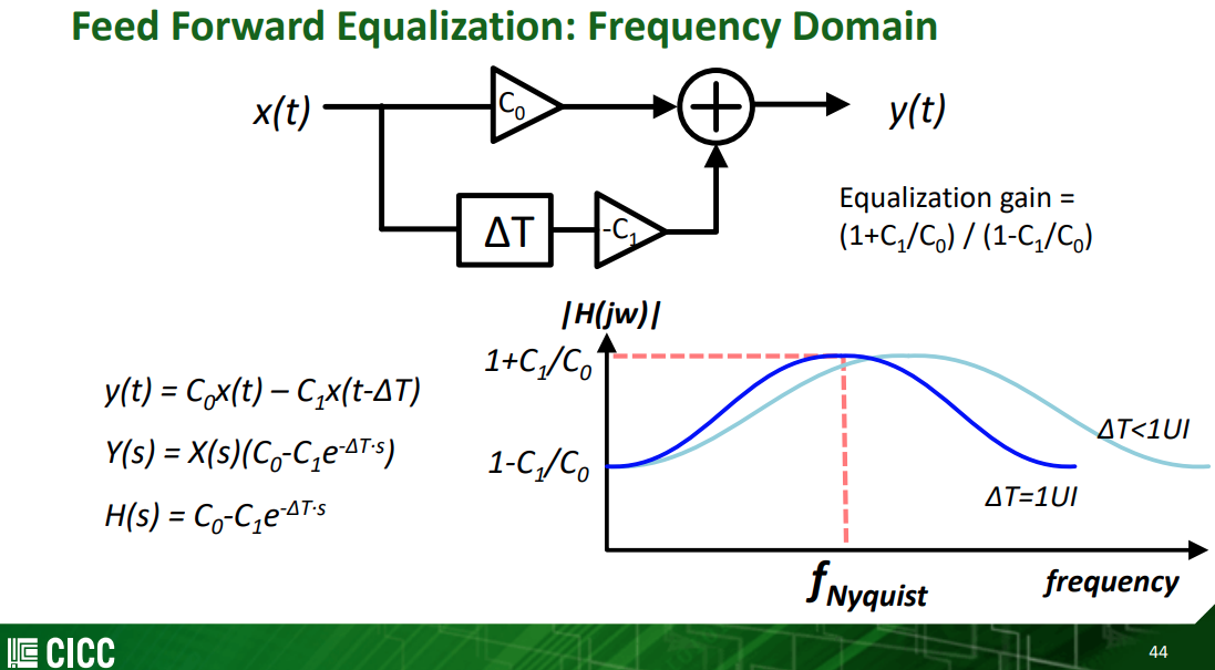 \[
x(t-\Delta T)\overset{FT}{\longrightarrow} X(s)e^{-\Delta T \cdot s}
\]
\[
x(t-\Delta T)\overset{FT}{\longrightarrow} X(s)e^{-\Delta T \cdot s}
\]
reference
Sam Palermo, ECEN720, Lecture 7: Equalization Introduction & TX FIR Eq
Sam Palermo, ECEN720, Lab5 –Equalization Circuits
B. Razavi, "The z-Transform for Analog Designers [The Analog Mind]," IEEE Solid-State Circuits Magazine, Volume. 12, Issue. 3, pp. 8-14, Summer 2020.
Jhwan Kim, CICC 2022, ES4-4: Transmitter Design for High-speed Serial Data Communications
Mathuranathan. Digital filter design – Introduction https://www.gaussianwaves.com/2020/02/introduction-to-digital-filter-design/