z-Transform & Laplace Transform
- Laplace transform
- a generalization of the continuous-time Fourier transform
- converts integro-differential equations into algebraic equations
- z-transforms
- a generalization of the discrete-time Fourier transform
- converts difference equations into algebraic equations
system function, transfer function: \(H(s)\)
frequency response: \(H(j\omega)\), if the ROC of \(H(s)\) includes the imaginary axis, i.e.\(s=j\omega \in \text{ROC}\)
Laplace Transform
To specify the Laplace transform of a signal, both the algebraic expression and the ROC are required. The ROC is the range of values of \(s\) for the integral of \(t\) converges
bilateral Laplace transform
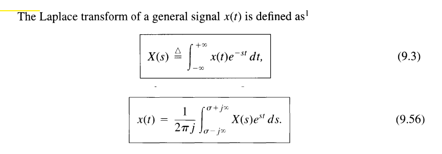
where \(s\) in the ROC and \(\mathfrak{Re}\{s\}=\sigma\)
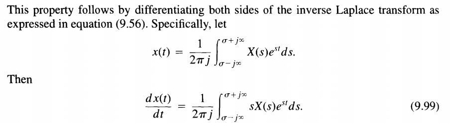
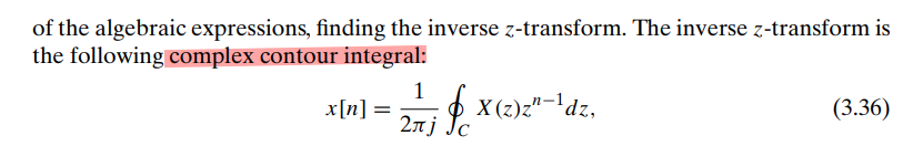
The formal evaluation of the integral for a general \(X(s)\) requires the use of contour integration in the complex plane. However, for the class of rational transforms, the inverse Laplace transform can be determined without directly evaluating eq. (9.56) by using the technique of partial fraction expansion
ROC Property
The range of values of s for which the integral in converges is referred to as the region of convergence (which we abbreviate as ROC) of the Laplace transform
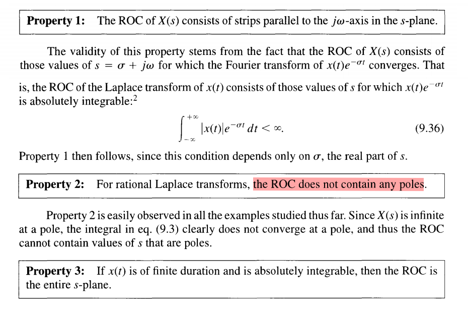
i.e. no pole in RHP for stable LTI sytem
System Causality
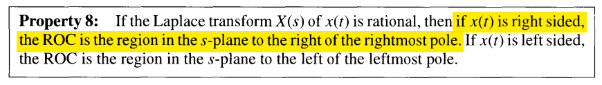
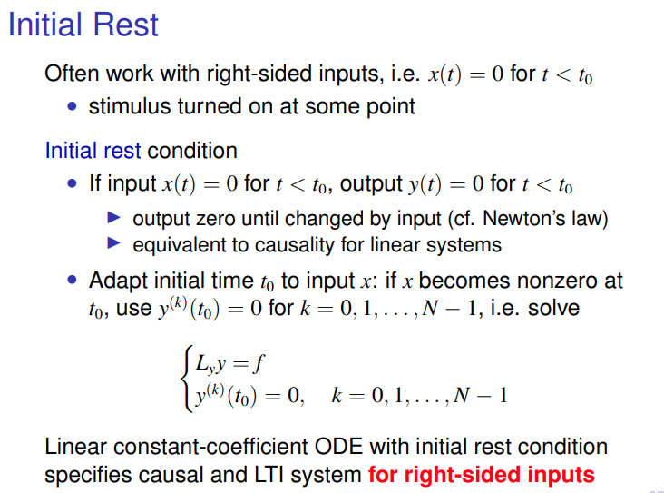
For a causal LTI system, the impulse response is zero for \(t \lt 0\) and thus is right sided

causality implies that the ROC is to the right of the rightmost pole, but the converse is not in general true, unless the system function is rational
System Stability
The system is stable, or equivalently, that \(h(t)\) is absolutely integrable and therefore has a Fourier transform, then the ROC must include the entire \(j\omega\)-axis


all of the poles have negative real parts
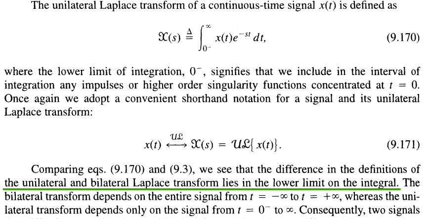
Unilateral Laplace transform
analyzing causal systems and, particularly, systems specified by linear constant-coefficient differential equations with nonzero initial conditions (i.e., systems that are not initially at rest)
A particularly important difference between the properties of the unilateral and bilateral transforms is the differentiation property \(\frac{d}{dt}x(t)\)
| Laplace Transform | |
|---|---|
| Bilateral Laplace Transform | \(sX(s)\) |
| Unilateral Laplace Transform | \(sX(s)-x(0^-)\) |
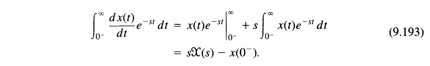
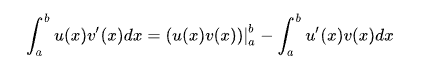
Integration by parts for unilateral Laplace transform
in Bilateral Laplace Transform
In fact, the initial- and final-value theorems are basically unilateral transform properties, as they apply only to signals \(x(t)\) that are identically \(0\) for \(t \lt 0\).
\(z\)-Transform
The \(z\)-transform for discrete-time signals is the counterpart of the Laplace transform for continuous-time signals
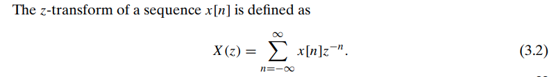
where \(z=re^{j\omega}\)
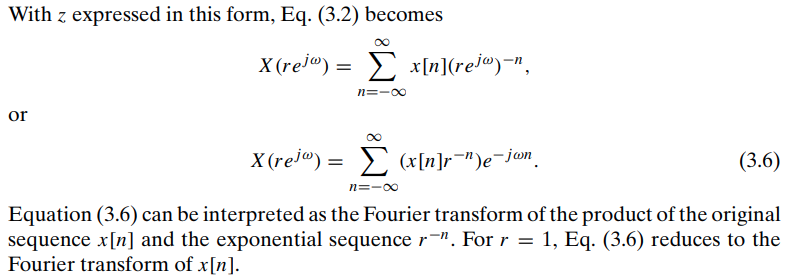
The \(z\)-transform evaluated on the unit circle corresponds to the Fourier transform
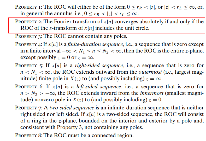
ROC Property
system stability
The system is stable, or equivalently, that \(h[n]\) is absolutely summable and therefore has a Fourier transform, then the ROC must include the unit circle
\(z\)-Transform Table
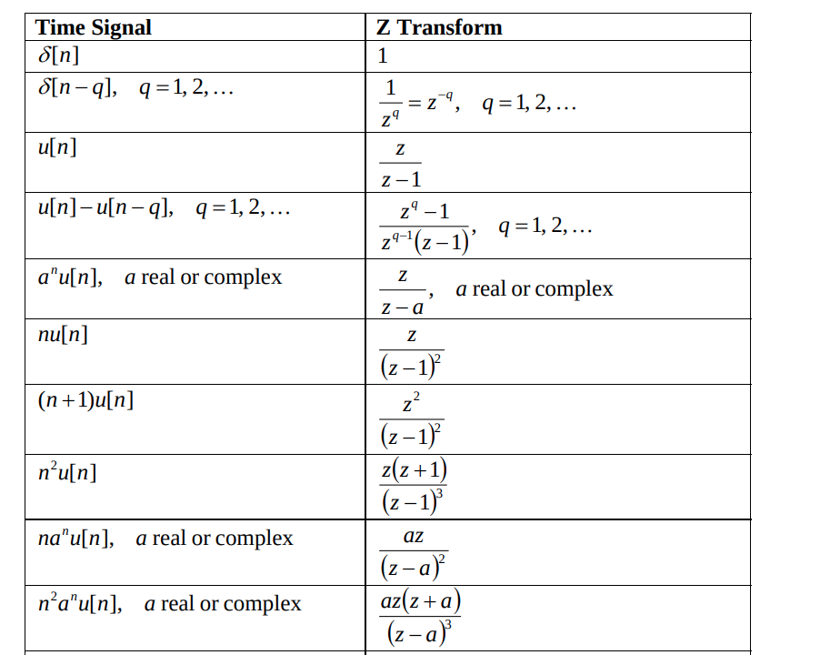
[http://www.ws.binghamton.edu/Fowler/fowler%20personal%20page/EE301_files/ZT%20Tables_rev2.pdf]
Unilateral \(z\)-Transform
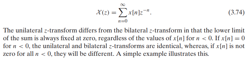
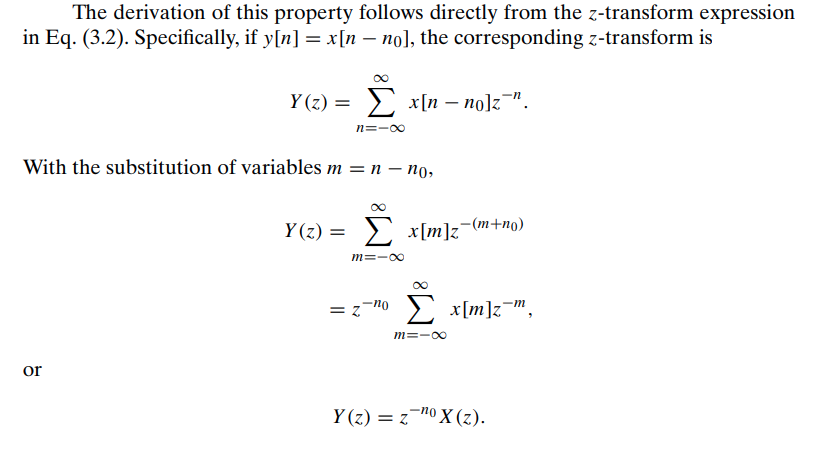
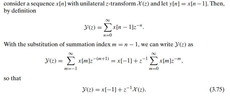
The time shifting property is different in the unilateral case because the lower limit in the unilateral transform definition is fixed at zero, \(x[n-n_0]\)
bilateral \(z\)-transform
unilateral \(z\)-transform
Initial rest condition
Initial Value Theorem & Final Value Theorem
Laplace Transform
Two valuable Laplace transform theorem
Initial Value Theorem, which states that it is always possible to determine the initial value of the time function \(f(t)\) from its Laplace transform \[ \lim _{s\to \infty}sF(s) = f(0^+) \]
Final Value Theorem allows us to compute the constant steady-state value of a time function given its Laplace transform \[ \lim _{s\to 0}sF(s) = f(\infty) \]
If \(f(t)\) is step response, then \(f(0^+) = H(\infty)\) and \(f(\infty) = H(0)\), where \(H(s)\) is transfer function
\(z\)-transform
Initial Value Theorem \[ f[0]=\lim_{z\to\infty}F(z) \] final value theorem \[ \lim_{n\to\infty}f[n]=\lim_{z\to1}(z-1)F(z) \]
Coert Vonk. Initial/final value proofs [https://coertvonk.com/physics/lfz-transforms/z/initial-final-value-proofs-31543]
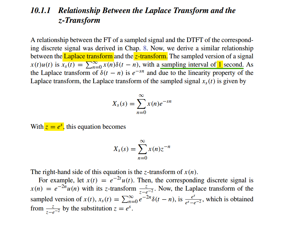
\(s\)- and \(z\)-Domains Connection
discrete-time systems also can be analyzed by means of the Laplace transform — the \(z\)-transform is the Laplace transform in disguise and that discrete-time systems can be analyzed as if they were continuous-time systems.
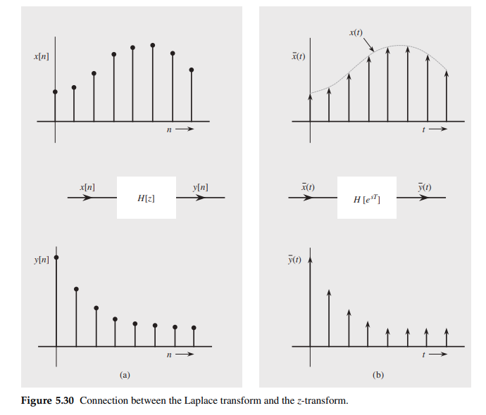
A continuous-time system with transfer function \(H(s)\) that is identical in structure to the discrete-time system \(H[z]\) except that the delays in \(H[z]\) are replaced by elements that delay continuous-time signals
delay element Time domain Transform \(z\)-transform \(\delta[n-1]\) \(z^{-1}\) Laplace transform \(\delta(t-T)\) \(e^{-sT}\)
| \(z\)-transform | Laplace transform | ||
|---|---|---|---|
| \(x[n]\) | \(X[z]=\sum_{n=0}^{\infty}x[n]z^{-n}\) | \(\bar{x}(t)=\sum_{n=0}^{\infty}x[n]\delta(t-nT)\) | \(\overline{X}(s)=\sum_{n=0}^{\infty}x[n]e^{-snT}\) |
| \(y[n]\) | \(Y[z]=\sum_{n=0}^{\infty}y[n]z^{-n}\) | \(\bar{y}(t)=\sum_{n=0}^{\infty}y[n]\delta(t-nT)\) | \(\overline{Y}(s)=\sum_{n=0}^{\infty}y[n]e^{-snT}\) |
| \(h[n]\) | \(H[z]=\sum_{n=0}^{\infty}h[n]z^{-n}\) | \(\bar{h}(t)=\sum_{n=0}^{\infty}h[n]\delta(t-nT)\) | \(\overline{H}(s)=\sum_{n=0}^{\infty}h[n]e^{-snT}\) |
| \(y[n]=x[n]*h[n]\) | \(Y[z]=X[z]H[z]\) | \(\bar{y}(t)=\bar{x}(t)*\bar{h}(t)\) | \(\overline{Y}(s)=\overline{X}(s)\overline{H}(s)\) |
Therefore, we obtain
\[\begin{align} \sum_{n=0}^{\infty}y[n]z^{-n} &=\sum_{n=0}^{\infty}x[n]z^{-n}\cdot\sum_{n=0}^{\infty}h[n]z^{-n} \\ \sum_{n=0}^{\infty}y[n]e^{-snT} &=\sum_{n=0}^{\infty}x[n]e^{-snT}\cdot \sum_{n=0}^{\infty}h[n]e^{-snT} \end{align}\]
The \(z\)-transform of a sequence can be considered to be the Laplace transform of impulses sampled train with a change of variable \(z = e^{sT}\) or \(s = \frac{1}{T}\ln z\)
Note that the transformation \(z = e^{sT}\) transforms the imaginary axis in the \(s\) plane (\(s = j\omega\)) into a unit circle in the \(z\) plane (\(z = e^{sT} = e^{j\omega T}\), or \(|z| = 1\))
Note: \(\bar{h}(t)\) is the impulse sampled version of \(h(t)\)
Note \(\bar{h}(t)\) is impulse sampled signal, whose CTFT is scaled by \(\frac{1}{T}\) of continuous signal \(h(t)\), \(\overline{H}[e^{sT}]=\overline{H}(e^{sT})\) is the approximation of continuous time system response, for example summation \(\frac{1}{1-z^{-1}}\) \[ \frac{1}{1-z^{-1}} = \frac{1}{1-e^{-sT}} \approx \frac{1}{j\omega \cdot T} \] And we know transform of integral \(u(t)\) is \(\frac{1}{s}\), as expected there is ratio \(T\)
Staszewski, Robert Bogdan, and Poras T. Balsara. All-digital frequency synthesizer in deep-submicron CMOS. John Wiley & Sons, 2006
D. Sundararajan. Signals and Systems A Practical Approach Second Edition, 2023
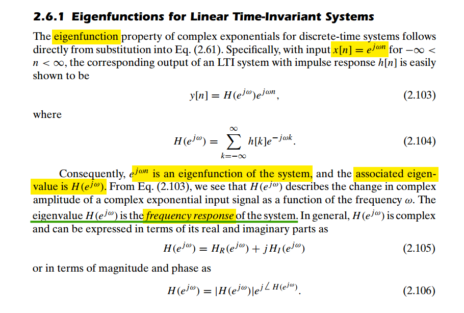
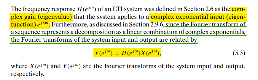
Frequency Response of Discrete-Time LTI Systems
Eugenio Schuster, Lehigh University, Discrete-Time Signal Analysis in the Frequency-Domain [https://www.lehigh.edu/~eus204/teaching/ME450_SIRC/notes/DTS_Tutorial.pdf]
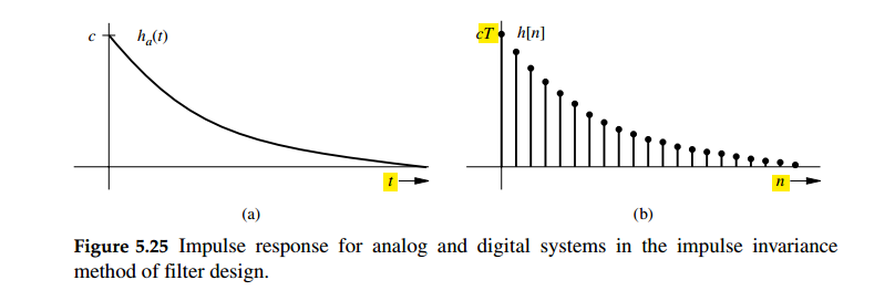
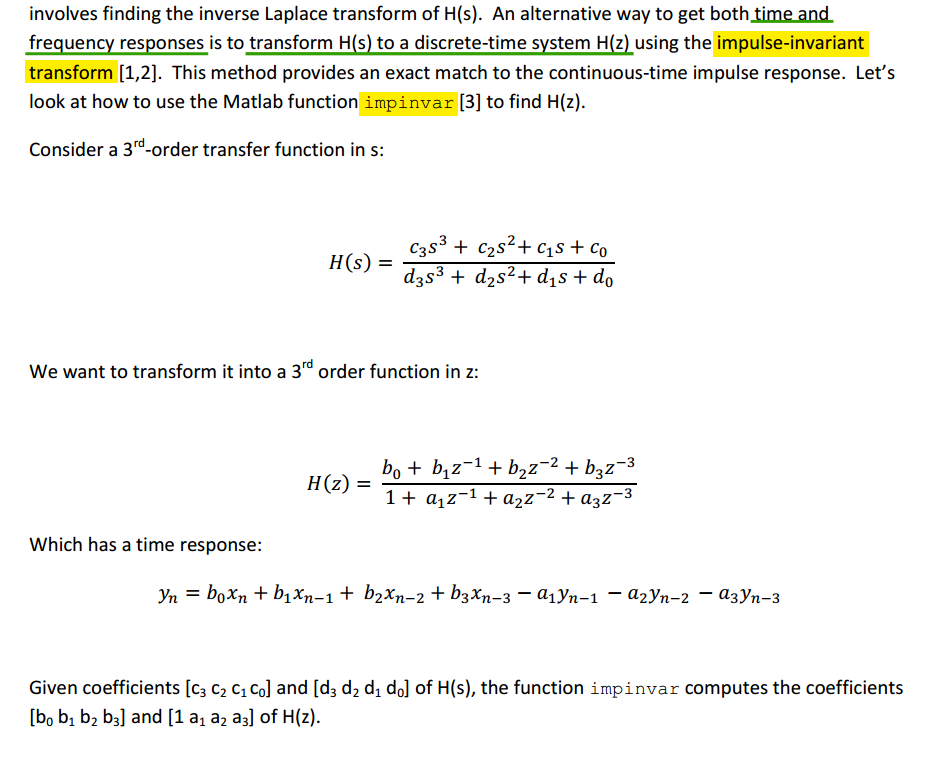
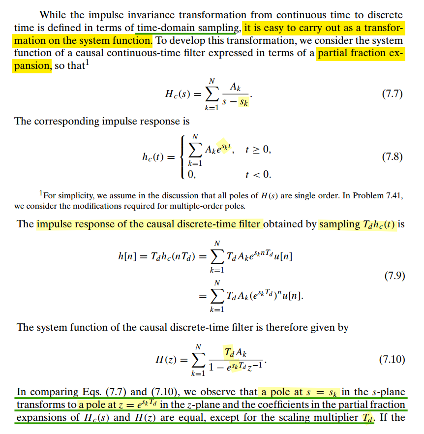
impulse invariance
A straightforward and useful relationship between the continuous-time impulse response \(h_c(t)\) and the discrete-time impulse response \(h[n]\)
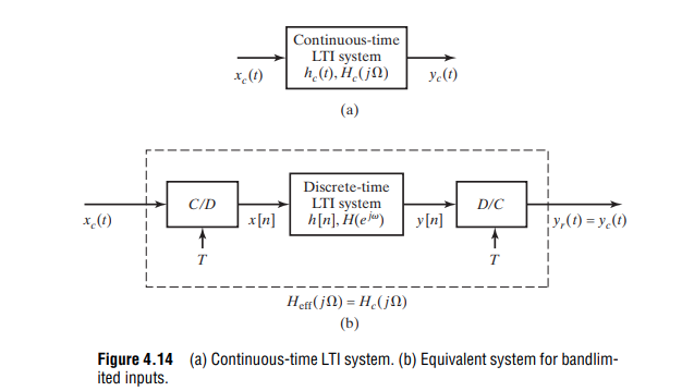
\[ h[n] = Th_c(nT) \]
and \(T\) is chosen such that
\[ H_c(j\omega)=0, \space\space |\hat{\omega}| \ge \frac{\pi}{T} \]
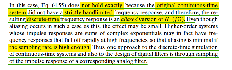
When \(h[n]\) and \(h_c(t)\) are related through the above equation, i.e., the impulse response of the discrete-time system is a scaled, sampled version of \(h_c(t)\), the discrete-time system is said to be an impulse-invariant version of the continuous-time system
we have \[ H(e^{j\hat{\omega}}) = H_c\left(j\frac{\hat{\omega}}{T}\right),\space\space |\hat{\omega}| \lt \pi \]
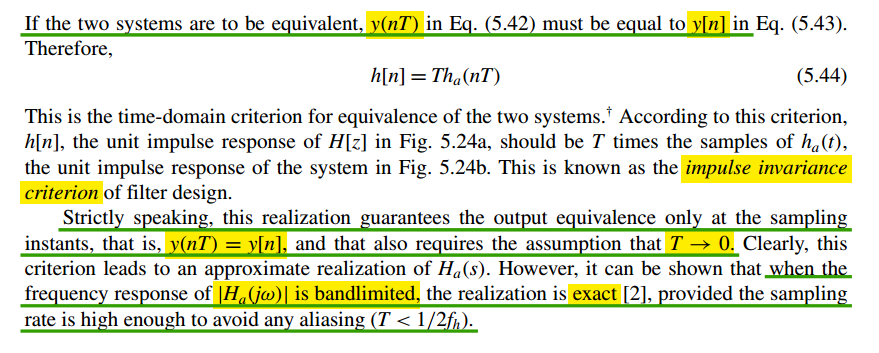
\(h[n] = Th_c(nT)\) and \(T\to 0\)
guarantees \(y_c(nT) = y_r(nT)\), i.e. output equivalence only at the sampling instants
\(H_c(j\Omega)\) is bandlimited and \(T \lt 1/2f_h\)
guarantees \(y_c(t) = y_r(t)\)
The scaling of \(T\) can alternatively be thought of as a normalization of the time domain, that is average impulse response shall be same i.e., \(h[n]\times 1 = h(nT)\times T\)
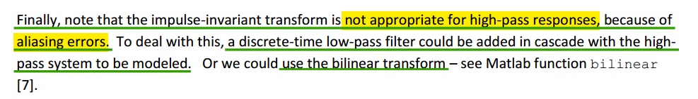
note that the impulse-invariant transform is not appropriate for high-pass responses, because of aliasing errors
⭐ bandlimited
⭐ bandlimited
Scale the Result if impulse not multiplied with \(T_s\)

[https://www.google.com.hk/search?q=matlab+continuous+transfer+function+in+time+domain+convolution]
1 | t = linspace(0, 10); |
Transfer function from sampled impulse response
continuous-time filter designs to discrete-time designs through techniques such as impulse invariance
useful functions
using
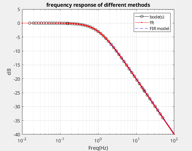
fftThe outputs of the DFT are samples of the DTFT
using
freqzmodeling as FIR filter, and the impulse response sequence of an FIR filter is the same as the sequence of filter coefficients, we can express the frequency response in terms of either the filter coefficients or the impulse response
fftis used infreqzinternally
freqzmethod is straightforward, which apply impulse invariance criteria. Thoughfftis used for signal processing mostly,
1 | clear all; |
!!! only multiply Ts
Neil Robertson. The Discrete Fourier Transform as a Frequency Response [https://www.dsprelated.com/showarticle/1498.php]
H(k) by using complex exponentials is indeed identical to the DFT of h(n)
H(f) by DFT ->
fftH(k) by using complex exponential ->
freqz
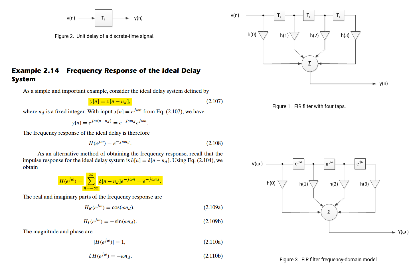
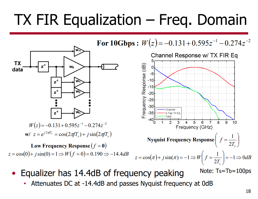
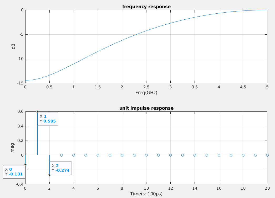
FIR Equalization
Frequency Response
 \[
z = e^{j\omega T_s}
\]
\[
z = e^{j\omega T_s}
\]
Unit impulse
filter coefficients are [-0.131, 0.595, -0.274] and sampling period is 100ps
1 | %% Frequency response |
impulse:For discrete-time systems, the impulse response is the response to a unit area pulse of length
Tsand height1/Ts, whereTsis the sample time of the system. (This pulse approaches \(\delta(t)\) asTsapproaches zero.)Scale output:
Multiply
impulseoutput with sample periodTsin order to correct1/Tsheight ofimpulsefunction.
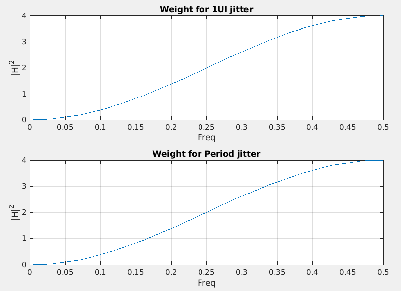
PSD transformation
If we have power spectrum or power spectrum density of both edge's absolute jitter (\(x(n)\)) , \(P_{\text{xx}}\)
Then 1UI jitter is \(x_{\text{1UI}}(n)=x(n)-x(n-1)\), and Period jitter is \(x_{\text{Period}}(n)=x(n)-x(n-2)\), which can be modeled as FIR filter, \(H(\omega) = 1-z^{-k}\), i.e. \(k=1\) for 1UI jitter and \(k=2\) Period jitter \[\begin{align} P_{\text{xx}}'(\omega) &= P_{\text{xx}}(\omega) \cdot \left| 1-z^{-k} \right|^2 \\ &= P_{\text{xx}}(\omega) \cdot \left| 1-(e^{j\omega T_s})^{-k} \right|^2 \\ &= P_{\text{xx}}(\omega) \cdot \left| 1-e^{-j\omega T_s k} \right|^2 \end{align}\]
1 | clear all |
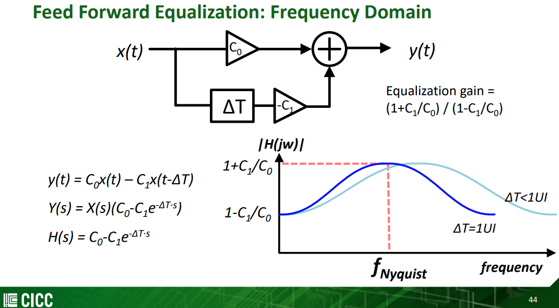 \[
x(t-\Delta T)\overset{FT}{\longrightarrow} X(s)e^{-\Delta T \cdot s}
\]
\[
x(t-\Delta T)\overset{FT}{\longrightarrow} X(s)e^{-\Delta T \cdot s}
\]
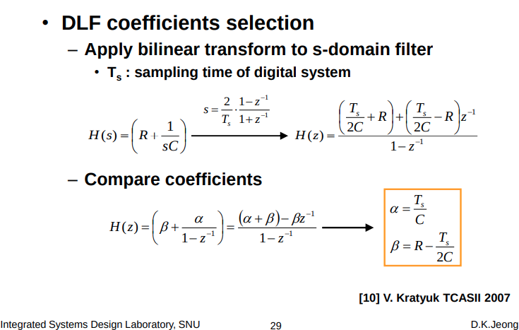
Bilinear Transform
The design of IIR filters (cont.) [https://ocw.mit.edu/courses/2-161-signal-processing-continuous-and-discrete-fall-2008/cc00ac6d468dc9dcf2238fc1d1a194d4_lecture_19.pdf]
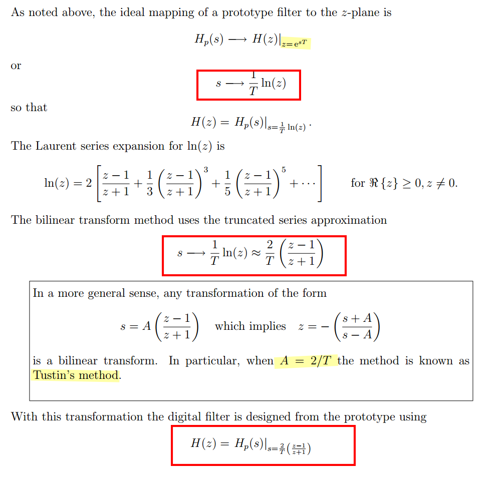
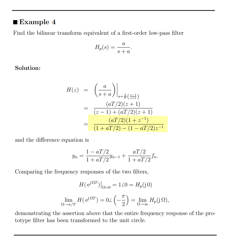
an algebraic transformation between the variables \(s\) and \(z\) that maps the entire imaginary \(j\Omega\)-axis in the \(s\)-plane to one revolution of the unit circle in the \(z\)-plane
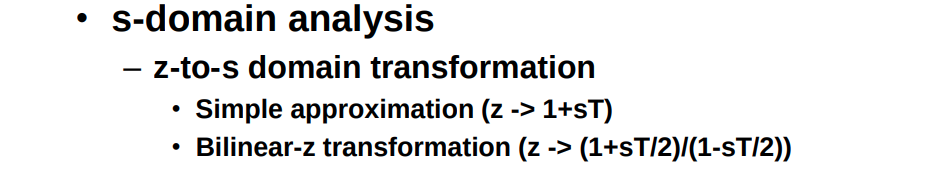
\[\begin{align} z &= \frac{1+s\frac{T_s}{2}}{1-s\frac{T_s}{2}} \\ s &= \frac{2}{T_s}\cdot \frac{1-z^{-1}}{1+z^{-1}} \end{align}\]
where \(T_s\) is the sampling period
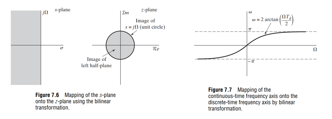
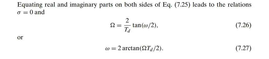
frequency warping:
The bilinear transformation avoids the problem of aliasing encountered with the use of impulse invariance, because it maps the entire imaginary axis of the \(s\)-plane onto the unit circle in the \(z\)-plane
impulse invariance cannot be used to map highpass continuous-time designs to high pass discrete-time designs, since highpass continuous-time filters are not bandlimited
Due to nonlinear warping of the frequency axis introduced by the bilinear transformation, bilinear transformation applied to a continuous-time differentiator will not result in a discrete-time differentiator. However, impulse invariance can be applied to bandlimited continuous-time differentiator
The feature of the frequency response of discrete-time differentiators is that it is linear with frequency
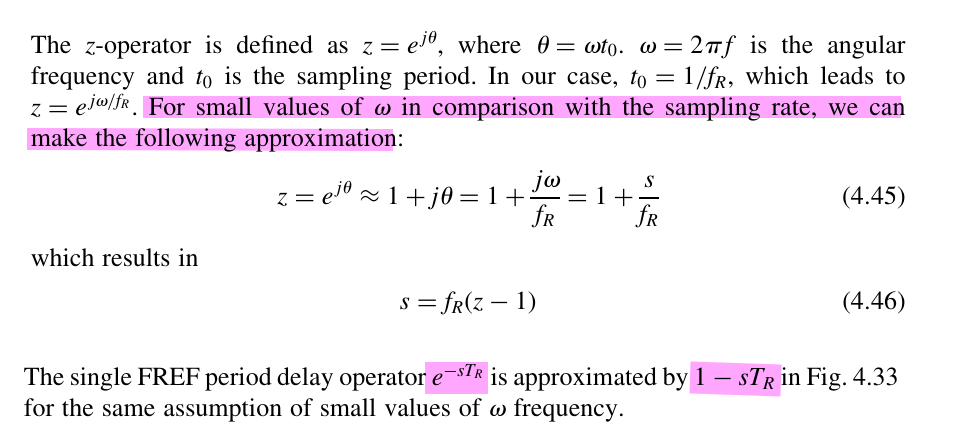
The simple approximation \(z=e^{sT}\approx1+sT\), the first
equal come from impulse invariance
essentially
Stephen Roberts. Lecture 3 - Design of Digital Filters [https://www.robots.ox.ac.uk/~sjrob/Teaching/B14_SP/b14_sp_lect3.pdf]
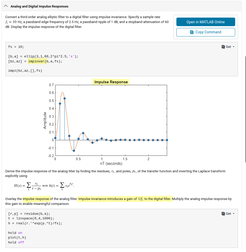
Design of IIR Filters From Analog Filters
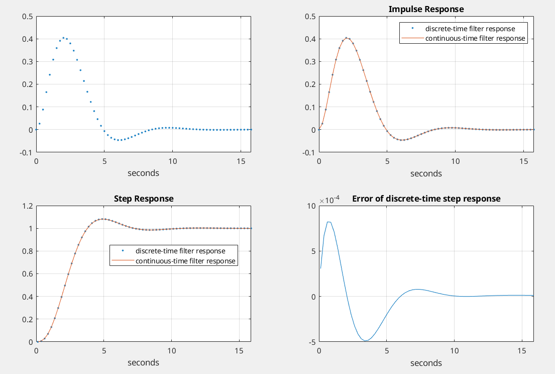
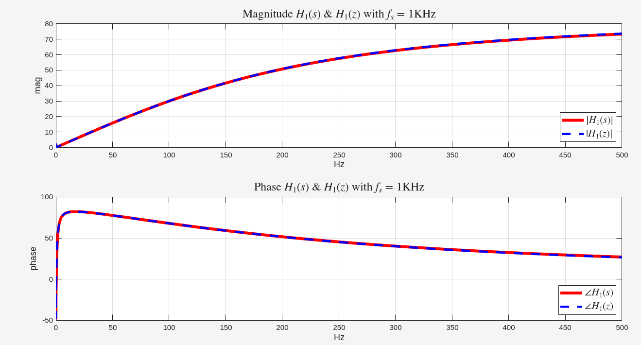
Modeling a Continuous-Time System with Matlab
Because the mapping between the continuous (\(s\)-plane) and discrete domains (\(z\)-plane) cannot be done exactly, the various design methods are at best approximations
Neil Robertson. Modeling a Continuous-Time System with Matlab [https://www.dsprelated.com/showarticle/1055.php]
—. Modeling Anti-Alias Filters [https://www.dsprelated.com/showarticle/1418.php]
impinvar[https://www.mathworks.com/help/signal/ref/impinvar.html]
bilinear[https://www.mathworks.com/help/signal/ref/bilinear.html]
filter[https://www.mathworks.com/help/matlab/ref/filter.html]
The design of IIR filters [https://ocw.mit.edu/courses/2-161-signal-processing-continuous-and-discrete-fall-2008/14f29be83ac38f11eb1a1bd5fdb6f5ea_lecture_18.pdf]
The design of IIR filters (cont.) [https://ocw.mit.edu/courses/2-161-signal-processing-continuous-and-discrete-fall-2008/cc00ac6d468dc9dcf2238fc1d1a194d4_lecture_19.pdf]
Lecture 19: Design of IIR Filters [http://smartdata.ece.ufl.edu/eee5502/2020_fall/media/2020_eee5502_slides28.pdf]
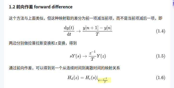
Derivatives Approximation
Perhaps the simplest method for low-order systems is to use backward-difference approximation to continuous domain derivatives
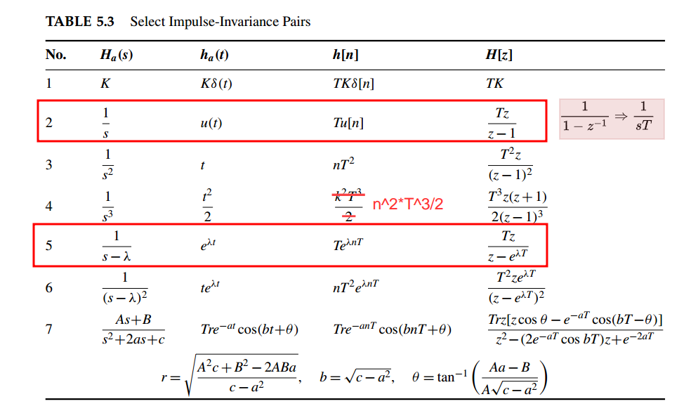
Note this approximation is not same with impulse invariance, e.g. \(\frac{1}{s^3} \to \frac{T^3z(z+1)}{2(-1)^3}\) employing impulse invariance
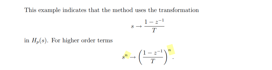
\[ 1- z^{-1} = 1-e^{-j\Omega T} = 1-\cos(\omega T) + j\sin(\Omega T) \approx 1-1+j\Omega T = s T \]
That is
\[ s \approx \frac{1-z^{-1}}{T} \]
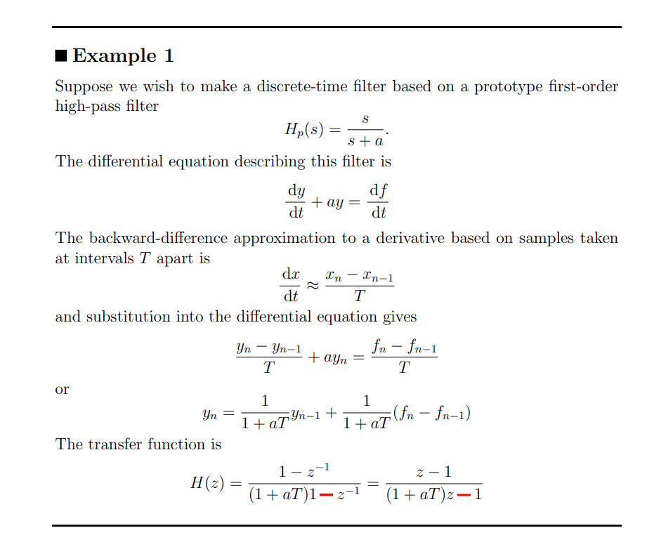
Suppose we wish to make a discrete-time filter based on a prototype first-order low-pass filter \[ H_p(s) = \frac{1}{s\tau + 1} \] The differential equation describing this filter is \[ \tau\frac{dy}{dt} + y = x \] then differential equation gives
\[ \tau\frac{y_n-y_{n-1}}{T} + y_n=x_n \] or \[ (\frac{\tau}{T}+1)y_n - \frac{\tau}{T}y_{n-1} = x_n \] The transfer function is \[ H(z) = \frac{\frac{T}{T+\tau}}{1-\frac{\tau}{T+\tau}z^{-1}} \]
or substitute \(s\) with \(\frac{1-z^{-1}}{T}\) into \(H_p(s)\) \[ H_p(z) = \frac{1}{\tau\frac{1-z^{-1}}{T} + 1} = \frac{\frac{T}{T+\tau}}{1-\frac{\tau}{T+\tau}z^{-1}}= \frac{\alpha}{1 +(\alpha -1)z^{-1}} \] where \(\alpha = \frac{T}{\tau+T}\)
Further, if time constants much longer than the time step \(\tau \gg T\) \[\begin{align} \frac{T}{T+\tau}& = \frac{T}{\tau}\cdot \frac{\tau}{T+\tau}\approx \frac{T}{\tau} \\ \frac{\tau}{T+\tau} &= \frac{\tau - T}{\tau}\cdot\frac{\tau^2}{\tau^2-T^2} \approx \frac{\tau - T}{\tau} = 1- \frac{T}{\tau} \end{align}\]
Then the first-order low pass filter \[ H_p(z) \approx \frac{ \frac{T}{\tau}}{1 +( \frac{T}{\tau} -1)z^{-1}} = \frac{\beta}{1 +(\beta -1)z^{-1}} \] where \(\beta = \frac{T}{\tau}\)
1 | # https://www.dsprelated.com/showarticle/1517/return-of-the-delta-sigma-modulators-part-1-modulation |
forward-difference approximation
模集王小桃. 连续时间滤波器到离散时间滤波器的映射 Mapping Continuous-Time Filters to Discrete-Time Filters [https://zhuanlan.zhihu.com/p/1961811157099746349]
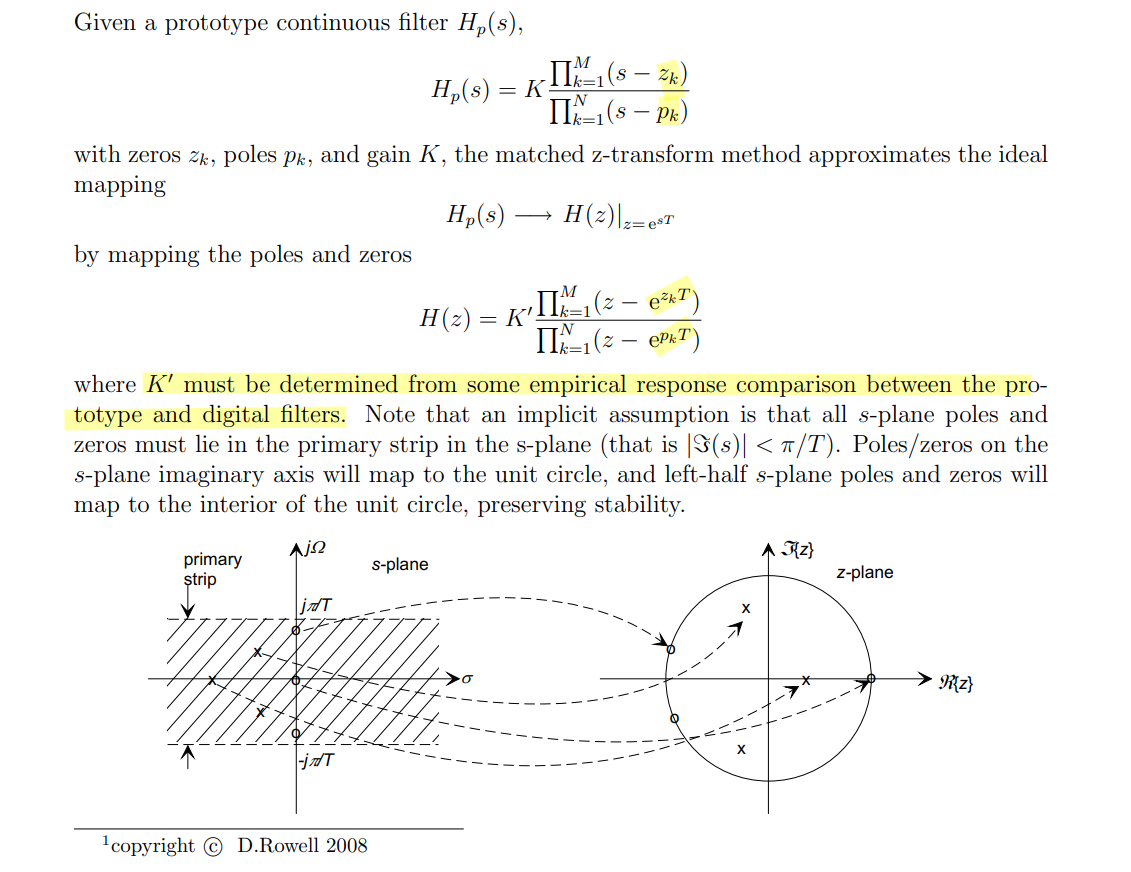
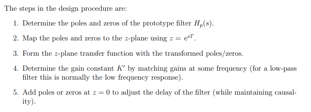
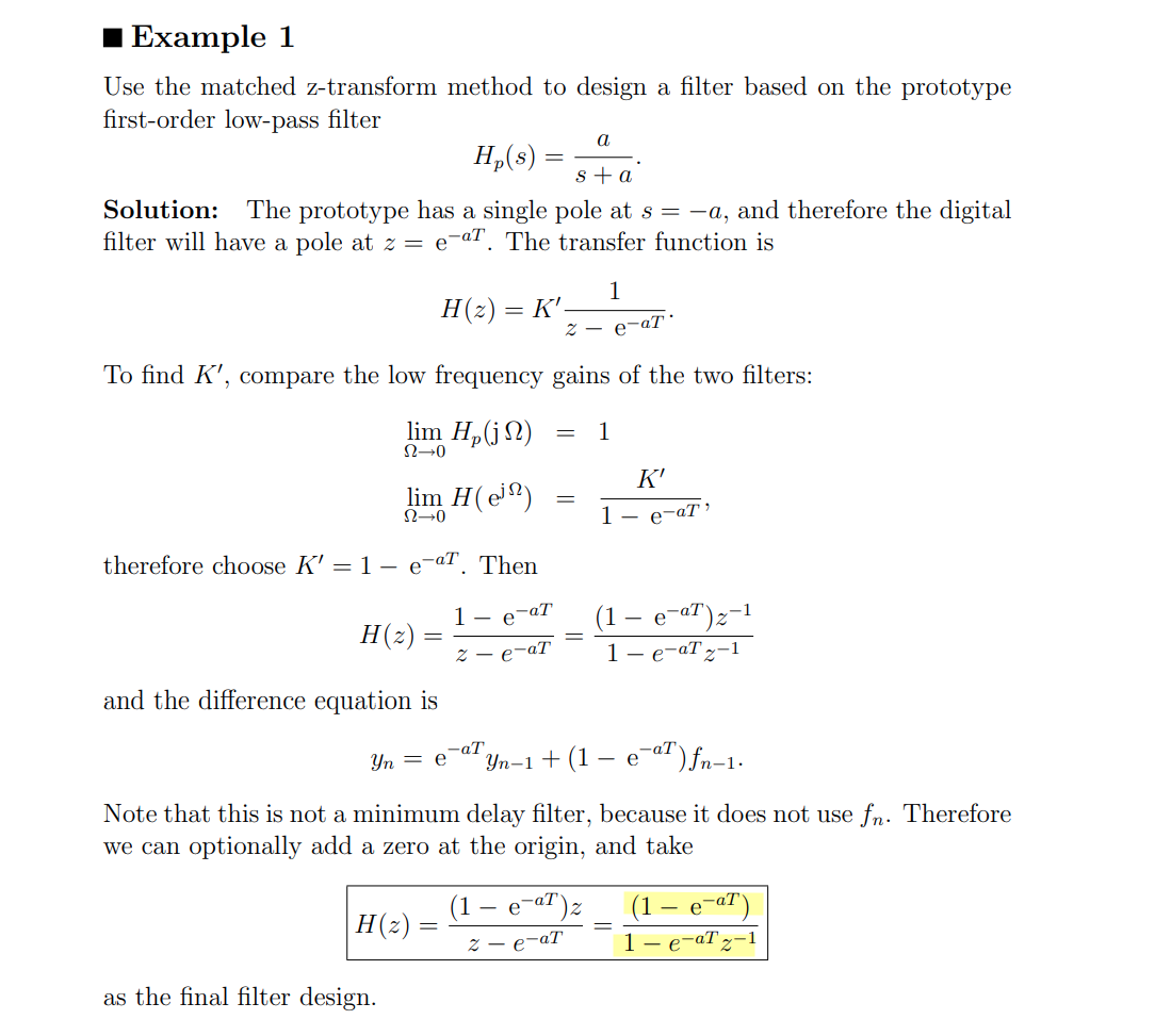
Matched z-Transform (Root Matching)
The matched Z-transform method, also called the pole-zero mapping or pole-zero matching method, and abbreviated MPZ or MZT
\[ z = e^{sT} \]
1 | % https://www.dsprelated.com/showarticle/1642.php |
Impulse Invariance
(impinvar)
- To extend the accurate frequency range, we would need to increase the sample rate
- impulse-invariant transform is not appropriate for high-pass responses, because of aliasing errors
Note \(h[n] = Th_c(nT)\), Multiply the analog impulse response by this gain to enable meaningful comparison (other response, like step, the amplitude correction is not needed)
1 | % https://www.dsprelated.com/showarticle/1055.php |
- To use the
filterfunction with thebcoefficients from an FIR filter, usey = filter(b,1,x).
Bilinear Transformation
(bilinear)
The Filter Wizard Substack: "Countdown to s-to-z…" [https://filterwizard.substack.com/p/countdown-to-s-to-z]
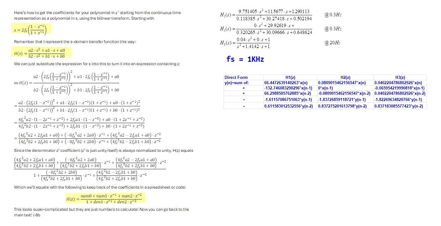
1 | a2 = 9.751405; a1 = 11.5677; a0 = 1.290113; |
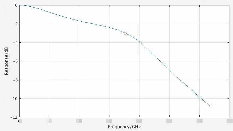
bandwidth from pulse response
L.W. Couch, Digital and Analog Communication Systems, 8th Edition, Pearson, 2013. [pdf]
Generating Basic signals – Rectangular Pulse and Power Spectral Density using FFT
Convolution Property of the Fourier Transform \[ x(t)*h(t)\longleftrightarrow X(\omega)H(\omega) \] pulse response can be obtained by convolve impulse response with UI length rectangular \[ H(\omega) = \frac{Y_{\text{pulse}}(\omega)}{X_{\text{rect}}(\omega)} = \frac{Y_{\text{pulse}}(\omega)}{\text{sinc}(\omega)} \]
1 | % Convolution Property of the Fourier Transform |
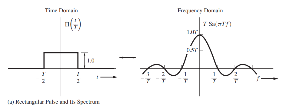
sinc function
Notice that the complete definition of \(\operatorname{sinc}\) on \(\mathbb R\) is \[ \operatorname{Sa}(x)=\operatorname{sinc}(x) = \begin{cases} \frac{\sin x}{x} & x\ne 0, \\ 1, & x = 0, \end{cases} \] which is continuous.
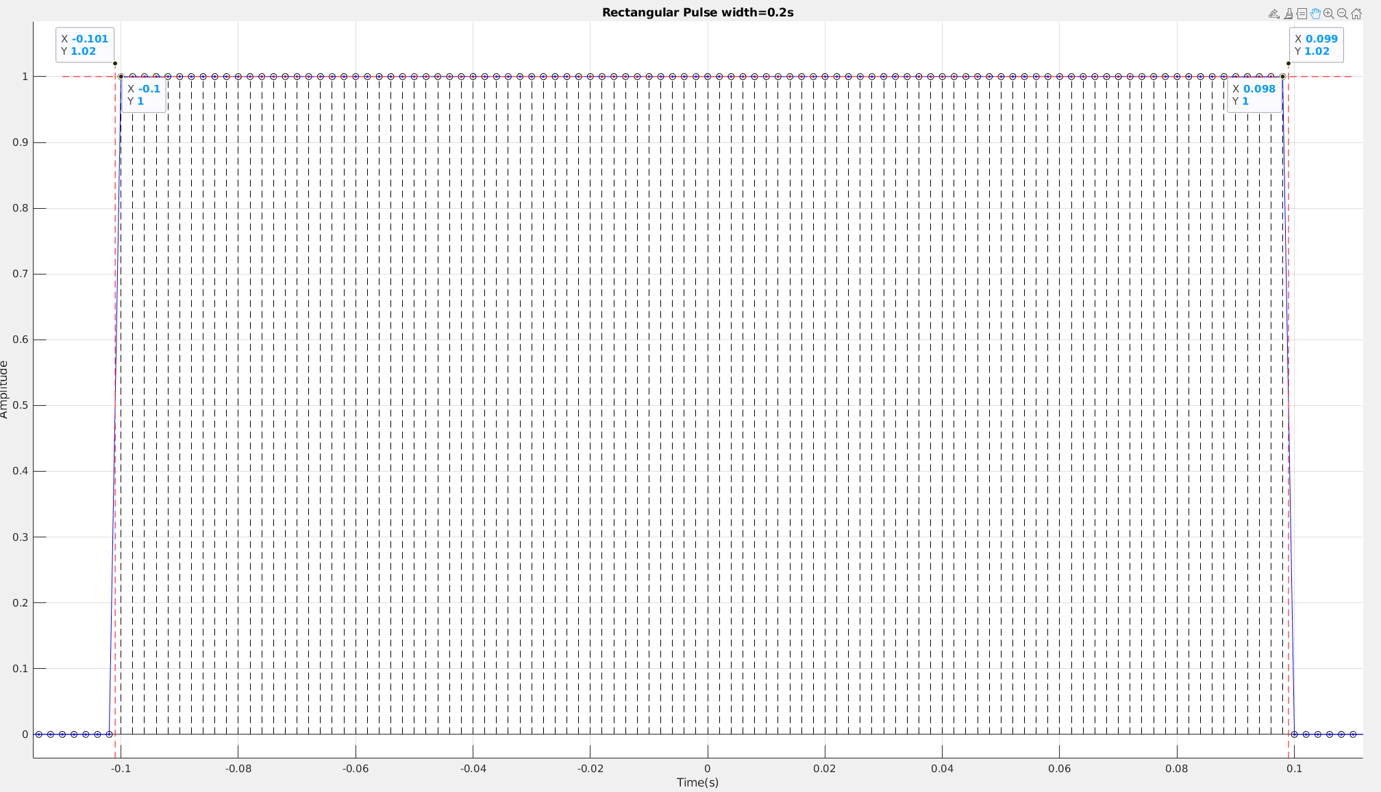
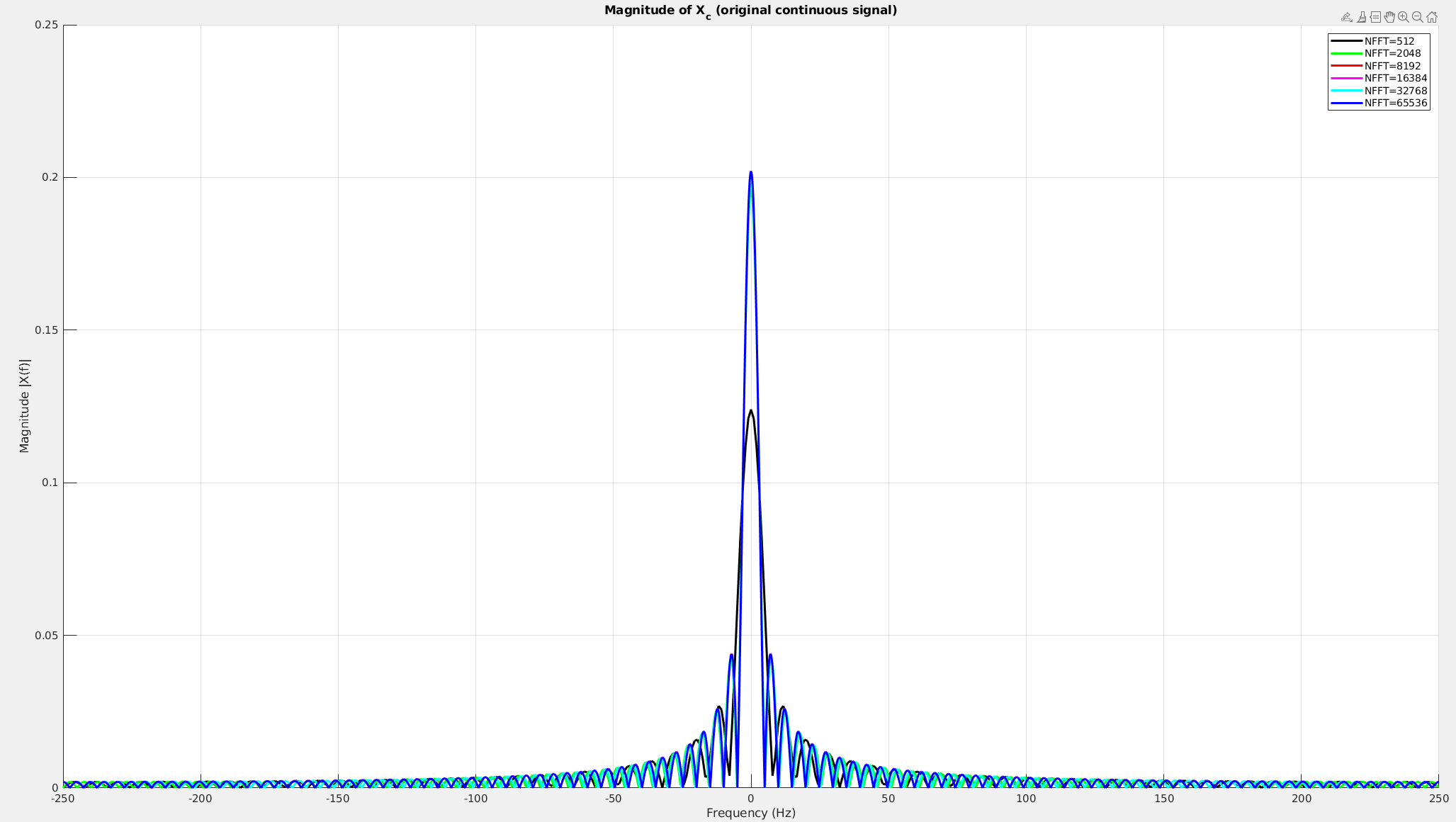
To approach to real spectrum of continuous rectangular waveform, \(\text{NFFT}\) has to be big enough.
1 | clear; |
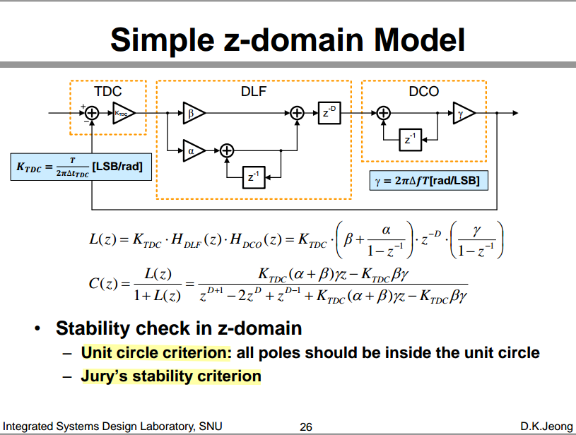
Stability check in z-domain
Unit circle criterion; Jury’s stability criterion
reference
Alan V. Oppenheim, Alan S. Willsky, and S. Hamid Nawab. 1996. Signals & systems (2nd ed.)
Alan V Oppenheim, Ronald W. Schafer. 2010. Discrete-Time Signal Processing, 3rd edition
B.P. Lathi, Roger Green. Linear Systems and Signals (The Oxford Series in Electrical and Computer Engineering) 3rd Edition
Sam Palermo, ECEN720, Lecture 7: Equalization Introduction & TX FIR Eq
Sam Palermo, ECEN720, Lab5 –Equalization Circuits
B. Razavi, "The z-Transform for Analog Designers [The Analog Mind]," IEEE Solid-State Circuits Magazine, Volume. 12, Issue. 3, pp. 8-14, Summer 2020. [https://www.seas.ucla.edu/brweb/papers/Journals/BR_SSCM_3_2020.pdf]
Jhwan Kim, CICC 2022, ES4-4: Transmitter Design for High-speed Serial Data Communications
Mathuranathan. Digital filter design – Introduction [https://www.gaussianwaves.com/2020/02/introduction-to-digital-filter-design/]
Daniel Boschen, "Fast Track to Designing FIR Filters with Python" [https://events.gnuradio.org/event/24/contributions/598/attachments/186/485/Boschen%20FIR%20Filter%20Presentation.pdf]
Daniel Boschen, "Quick Start on Control Loops with Python" [https://events.gnuradio.org/event/24/contributions/599/attachments/187/480/Boschen%20Control%20Presentation.pdf]