Power Spectra and Power Spectral Densities
One will see the following phenomena:
- A power spectrum is equal to the square of the absolute value of DFT.
- The sum of all power spectral lines in a power spectrum is equal to the power of the input signal.
- The integral of a PSD is equal to the power of the input signal.
power spectrum has units of \(V^2\) and power spectral density has units of \(V^2/Hz\)
Parseval's theorem is a property of the Discrete Fourier Transform (DFT) that states: \[ \sum_{n=0}^{N-1}|x(n)|^2 = \frac{1}{N}\sum_{k=0}^{N-1}|X(k)|^2 \] Multiply both sides of the above by \(1/N\): \[ \frac{1}{N}\sum_{n=0}^{N-1}|x(n)|^2 = \frac{1}{N^2}\sum_{k=0}^{N-1}|X(k)|^2 \] \(|x(n)|^2\) is instantaneous power of a sample of the time signal. So the left side of the equation is just the average power of the signal over the N samples. \[ P_{\text{av}} = \frac{1}{N^2}\sum_{k=0}^{N-1}|X(k)|^2\text{, }V^2 \] For the each DFT bin, we can say: \[ P_{\text{bin}}(k) = \frac{1}{N^2}|X(k)|^2\text{, k=0:N-1, }V^2/\text{bin} \] This is the power spectrum of the signal.
Note that \(X(k)\) is the two-sided spectrum. If \(x(n)\) is real, then \(X(k)\) is symmetric about \(fs/2\), with each side containing half of the power. In that case, we can choose to keep just the one-sided spectrum, and multiply Pbin by 2 (except DC & Nyquist):
\[ P_{\text{bin,one-sided}}(k) = \left\{ \begin{array}{cl} \frac{1}{N^2}|X(0)|^2 & : \ k = 0 \\ \frac{2}{N^2}|X(k)|^2 & : \ 1 \leq k \leq N/2-1 \\ \frac{1}{N^2}|X(N/2)|^2 & : \ k = N/2 \end{array} \right. \]
1 | rng default |
where xsq_sum_avg is same with
specsq_sum_avg
For a discrete-time sequence x(n), the DFT is defined as: \[ X(k) = \sum_{n=0}^{N-1}x(n)e^{-j2\pi kn/N} \] By it definition, the DFT does NOT apply to infinite duration signals.
scaling DFT results
| spectra type | unit |
|---|---|
| amplitude spectrum | V |
| power spectrum | V^2 |
| power spectrum density | V^2/Hz |
[https://github.com/AppliedAcousticsChalmers/scaling-of-the-dft]
Different scaling is needed to apply for amplitude spectrum, power spectrum and power spectrum density, which shown as below
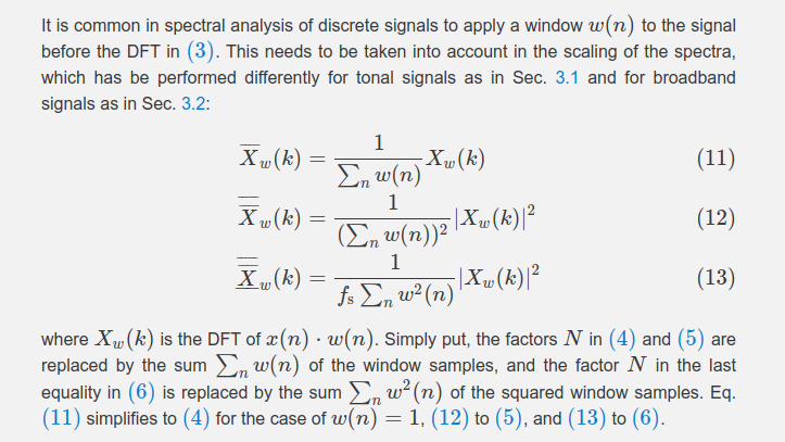
\(f_s\) in Eq.(13) is sample rate rather than frequency resolution.
And Eq.(13) can be expressed as \[ \text{PSD}(k) =\frac{1}{f_{\text{res}}\cdot N\sum_{n}w^2(n)}\left|X_{\omega}(k)\right|^2 \] where \(f_{\text{res}}\) is frequency resolution
We define the following two sums for normalization purposes:
\[\begin{align} S_1 &= \sum_{j=0}^{N-1}w_j \\ S_2 &= \sum_{j=0}^{N-1}w_j^2 \end{align}\]
Given Eq.(12) and Eq.(13) \[\begin{align} \text{PS(k)} &= \text{PSD(k)} \cdot \frac{f_s \sum_{n}w^2(n)}{(\sum_{n}\omega(n))^2} \\ &= \text{PSD(k)} \cdot f_{\text{res}} \cdot \frac{N \sum_{n}w^2(n)}{(\sum_{n}w(n))^2} \\ &= \text{PSD(k)} \cdot f_{\text{res}} \cdot \frac{N S_2}{S_1^2} \\ &= \text{PSD(k)} \cdot f_{\text{res}} \cdot \text{NENBW} \\ &= \text{PSD(k)} \cdot \text{ENBW} \end{align}\]
where Normalized Equivalent Noise BandWidth is defined as \[ \text{NENBW} =\frac{N S_2}{S_1^2} \] and Effective Noise BandWidth is \[ \text{ENBW} =f_{\text{res}} \cdot \frac{N S_2}{S_1^2} \]
For Rectangular window, \(\text{ENBW} =f_{\text{res}}\)
This equivalent noise bandwidth is required when the resulting spectrum is to be expressed as spectral density (such as for noise measurements).
Eq.(13) Example:
1 | Fs = 1024; |
window effects
It is possible to correct both the amplitude and energy content of the windowed signal to equal the original signal. However, both corrections cannot be applied simultaneously
Amplitude correction
Linear (amplitude) Spectrum \[ X(k) = \frac{X_{\omega}(k)}{S_1} \] power spectrum \[ \text{PS}=\frac{\left| X_{\omega}(k) \right|^2}{S_1^2} \]
usage: tone amplitude
Power correction
power spectral density (PSD) \[ \text{PSD} =\frac{\left|X_{\omega}(k)\right|^2}{f_s\cdot S_2} \]
We have \(\text{PSD} = \frac{\text{PS}}{\text{ENBW}}\), where \(\text{ENBW}=\frac{N \cdot S_2}{S_1^2}f_{\text{res}}\)
linear power spectrum \[ \text{PS}_L=\frac{|X_{\omega}(k)|^2}{N\cdot S_2} \]
usage: RMS value, total power \[ \text{PS}_L(k)=\text{PSD(k)} \cdot f_{\text{res}} \]
Window Correction Factors
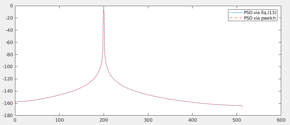
While a window helps reduce leakage (The window reduces the jumps at the ends of the repeated signal), the window itself distorts the data in two different ways:
Amplitude – The amplitude of the signal is reduced
This is due to the fact that the window removes information in the signal
Energy – The area under the curve, or energy of the signal, is reduced
Window correction factors are used to try and compensate for the effects of applying a window to data. There are both amplitude and energy correction factors.
| Window Type | Amplitude Correction (\(K_a\)) | Energy Correction (\(K_e\)) |
|---|---|---|
| Rectangluar | 1.0 | 1.0 |
| hann | 1.9922 | 1.6298 |
| blackman | 2.3903 | 1.8155 |
| kaiser | 1.0206 | 1.0204 |
Only the Uniform window (rectangular window), which is equivalent to no window, has the same amplitude and energy correction factors.
\[\begin{align} X(k) &= \frac{X_\omega(k)}{\sum_n w(n)} \\ &= \frac{N}{\sum_n w(n)} \frac{X_\omega(k)}{N} \\ &= K_a \cdot \frac{X_\omega(k)}{N} \end{align}\] where \(K_a = \frac{N}{\sum_n \omega(n)}\)
In literature, Coherent power gain is defined show below, which is close related to \(K_a\) \[ \text{Coherent power gain (dB)} = 20 \; log_{10} \left( \frac{\sum_n w[n]}{N} \right) \]
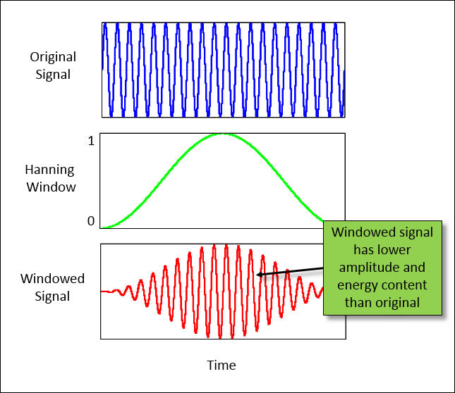
With amplitude correction, by multiplying by two, the peak value of both the original and corrected spectrum match. However the energy content is not the same.
The amplitude corrected signal (red) appears to have more energy, or area under the curve, than the original signal (blue).
\[\begin{align} \text{PSD} &=\frac{1}{f_{\text{res}}\cdot N\sum_{n}w^2(n)}\left|X_{\omega}(K)\right|^2 \\ &= \frac{N}{\sum_{n}w^2(n)} \frac{\left|X_{\omega}(K)\right|^2}{f_{\text{res}}\cdot N^2} \\ &=\left|K_e \cdot \frac{X_{\omega}(K)}{N}\right|^2 \cdot \frac{1}{f_{\text{res}}} \end{align}\]
wherer \(K_e = \sqrt{\frac{N}{\sum_{n}\omega^2(n)}}\)
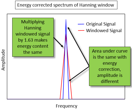
Multiplying the values in the spectrum by 1.63, rather than 2, makes the area under the curve the same for both the original signal (blue) and energy corrected signal (red)
hanning's correction factors:
1 | N = 256; |
1 | Ka = |
Amplitude,Power Correction Example
1 | %% 200 Hz, amplitude 1 and 200/3 Hz amplitude 0.3 |
1 | xrms0: 0.7383 |
RMS
We may also want to know for example the RMS value of the signal, in order to know how much power the signal generates. This can be done using Parseval’s theorem.
For a periodic signal, which has a discrete spectrum, we obtain its total RMS value by summing the included signals using \[ x_{\text{rms}}=\sqrt{\sum R_{xk}^2} \] Where \(R_{xk}\) is the RMS value of each sinusoid for \(k=1,2,3,...\) The RMS value of a signal consisting of a number of sinusoids is consequently equal to the square root of the sum of the RMS values.
This result could also be explained by noting that sinusoids of different frequencies are orthogonal, and can therefore be summed like vectors (using Pythagoras’ theorem)
For a random signal we cannot interpret the spectrum in the same way. As we have stated earlier, the PSD of a random signal contains all frequencies in a particular frequency band, which makes it impossible to add the frequencies up. Instead, as the PSD is a density function, the correct interpretation is to sum the area under the PSD in a specific frequency range, which then is the square of the RMS, i.e., the mean-square value of the signal \[ x_{\text{rms}}=\sqrt{\int G_{xx}(f)df}=\sqrt{\text{area under the curve}} \] The linear spectrum, or RMS spectrum, defined by \[\begin{align} X_L(k) &= \sqrt{\text{PSD(k)} \cdot f_{\text{res}}}\\ &=\sqrt{\frac{\left|X_{\omega}(k)\right|^2}{f_{\text{res}}\cdot N\sum_{n}\omega^2(n)} \cdot f_{\text{res}}} \\ &= \sqrt{\frac{\left|X_{\omega}(k)\right|^2}{N\sum_{n}\omega^2(n)}} \\ &= \sqrt{\frac{|X_{\omega}(k)|^2}{N\cdot S_2}} \end{align}\]
The corresponding linear power spectrum or RMS power spectrum can be defined by \[\begin{align} \text{PS}_L(k)&=X_L(k)^2=\frac{|X_{\omega}(k)|^2}{S_1^2}\frac{S_1^2}{N\cdot S_2} \\ &=\text{PS}(k) \cdot \frac{S_1^2}{N\cdot S_2} \end{align}\]
So, RMS can be calculated as below \[\begin{align} P_{\text{tot}} &= \sum \text{PS}_L(k) \\ \text{RMS} &= \sqrt{P_{\text{tot}}} \end{align}\]
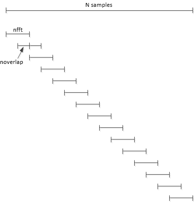
DFT averaging
we use \(N= 8*\text{nfft}\) time
samples of \(x\) and set the number of
overlapping samples to \(\text{nfft}/2 =
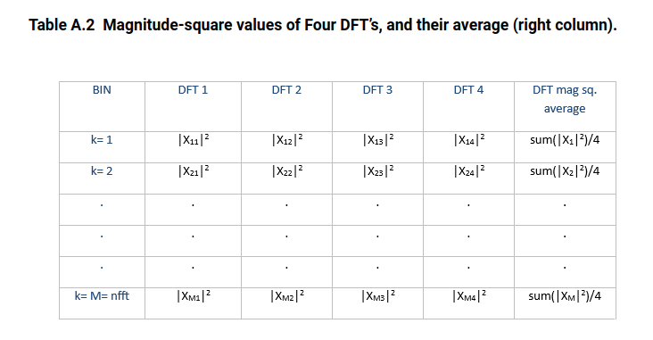
512\). pwelch takes the DFT of \(\text{Navg} = 15\) overlapping segments of
\(x\), each of length \(\text{nfft}\), then averages the \(|X(k)|^2\) of the DFT’s.
In general, if there are an integer number of segments that cover all samples of N, we have \[ N = (N_{\text{avg}}-1)*D + \text{nfft} \] where \(D=\text{nfft}-\text{noverlap}\). For our case, with \(D = \text{nfft}/2\) and \(N/\text{nfft} = 8\), we have \[ N_{\text{avg}}=2*N/\text{nfft}-1=15 \] For a given number of time samples N, using overlapping segments lets us increase \(N_{avg}\) compared with no overlapping. In this case, overlapping of 50% increases \(N_{avg}\) from 8 to 15. Here is the Matlab code to compute the spectrum:
1 | nfft= 1024; |
DFT averaging reduces the variance \(\sigma^2\) of the noise spectrum by a factor of \(N_{avg}\), as long as
noverlapis not greater thannfft/2
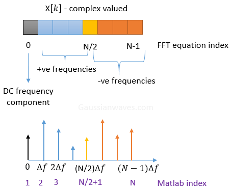
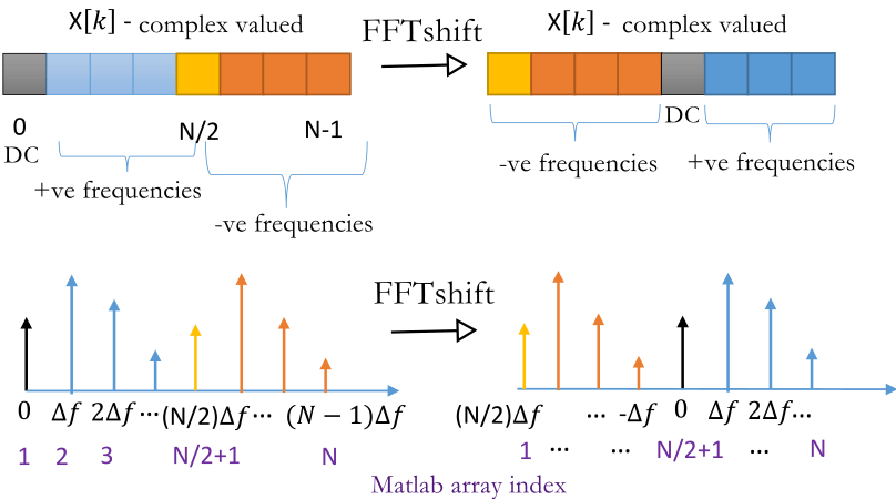
fftshift
The result of fft and its index is shown as below
After fftshift
1 | >> fftshift([0 1 2 3 4 5 6 7]) |
1 | clear; |
dft and
psd function in virtuoso
dftalways return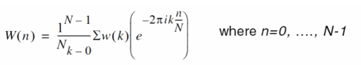
To compensate windowing effect, \(W(n)\), the dft output should
be multiplied by \(K_a\), e.g. 1.9922
for hanning window.
psdfunction has taken into account \(K_e\), postprocessing is not needed
reference
Heinzel, Gerhard, A. O. Rüdiger and Roland Schilling. "Spectrum and spectral density estimation by the Discrete Fourier transform (DFT), including a comprehensive list of window functions and some new at-top windows." (2002). URL: https://holometer.fnal.gov/GH_FFT.pdf
mathworks, Power Spectral Density Estimates Using FFT
Lyons, Richard, “Widowing Functions Improve FFT Results”, EDN, June 1, 1998. https://www.edn.com/electronics-news/4383713/Windowing-Functions-Improve-FFT-Results-Part-I
Rapuano, Sergio, and Harris, Fred J., An Introduction to FFT and Time Domain Windows, IEEE Instrumentation and Measurement Magazine, December, 2007. https://ieeexplore.ieee.org/document/4428580
Neil Robertson, The Power Spectrum
—, Use Matlab Function pwelch to Find Power Spectral Density – or Do It Yourself
—, Evaluate Window Functions for the Discrete Fourier Transform
—. Add a Power Marker to a Power Spectral Density (PSD) Plot [https://www.dsprelated.com/showarticle/1387.php]
Mathuranathan Viswanathan, Interpret FFT, complex DFT, frequency bins & FFTShift
robert bristow-johnson, Does windowing affect Parseval's theorem?
Window Correction Factors URL: https://community.sw.siemens.com/s/article/window-correction-factors
Brandt, A, 2011. Noise and vibration analysis: signal analysis and experimental procedures. John Wiley & Sons
What should be the correct scaling for PSD calculation using fft. URL:https://dsp.stackexchange.com/a/32205
POWER SPECTRAL DENSITY CALCULATION VIA MATLAB Revision C. URL: http://www.vibrationdata.com/tutorials_alt/psd_mat.pdf
Jens Ahrens, Carl Andersson, Patrik Höstmad, Wolfgang Kropp, “Tutorial on Scaling of the Discrete Fourier Transform and the Implied Physical Units of the Spectra of Time-Discrete Signals” in 148th Convention of the AES, e-Brief 56, May 2020 [ pdf, web ].
Manolakis, D., & Ingle, V. (2011). Applied Digital Signal Processing: Theory and Practice. Cambridge: Cambridge University Press. doi:10.1017/CBO9780511835261