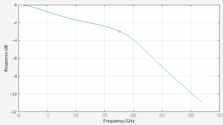
How to obtain channel bandwidth from pulse response
Convolution Property of the Fourier Transform \[ x(t)*h(t)\longleftrightarrow X(\omega)H(\omega) \] pulse response can be obtained by convolve impulse response with UI length rectangular \[ H(\omega) = \frac{Y_{\text{pulse}}(\omega)}{X_{\text{rect}}(\omega)} = \frac{Y_{\text{pulse}}(\omega)}{\text{sinc}(\omega)} \]
1 | % Convolution Property of the Fourier Transform |
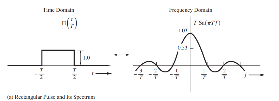
sinc function
Notice that the complete definition of \(\operatorname{sinc}\) on \(\mathbb R\) is \[ \operatorname{Sa}(x)=\operatorname{sinc}(x) = \begin{cases} \frac{\sin x}{x} & x\ne 0, \\ 1, & x = 0, \end{cases} \] which is continuous.
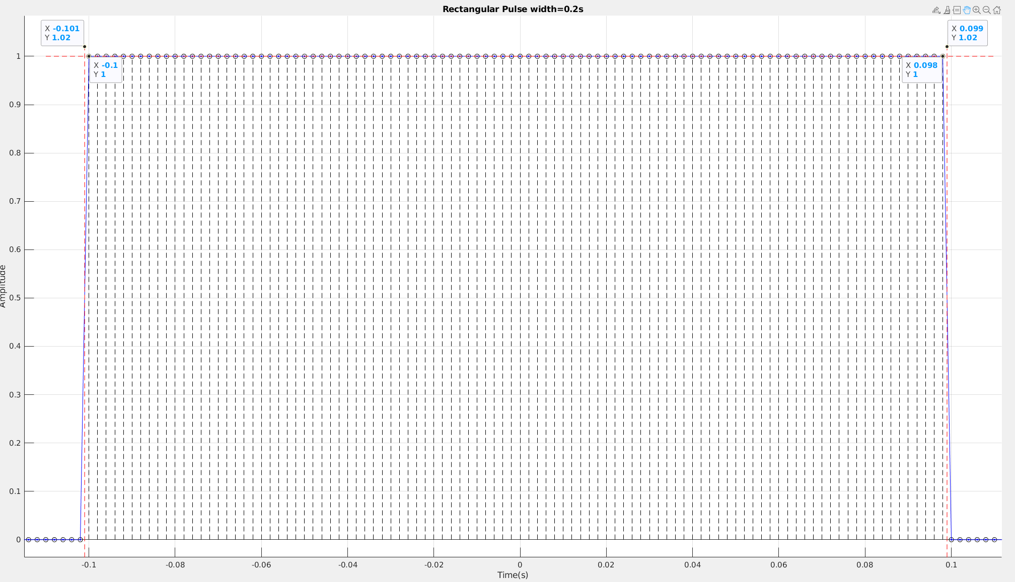
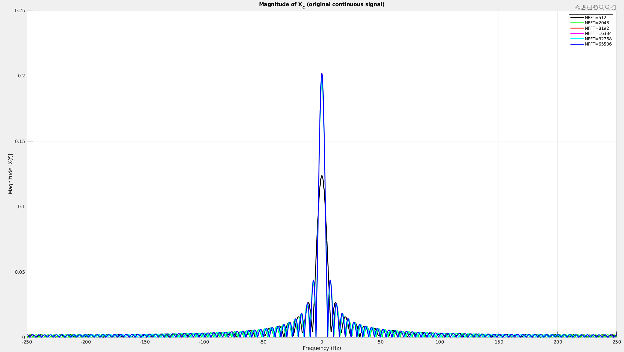
To approach to real spectrum of continuous rectangular waveform, \(\text{NFFT}\) has to be big enough.
1 | clear; |
reference
L.W. Couch, Digital and Analog Communication Systems, 8th Edition, Pearson, 2013.
Generating Basic signals – Rectangular Pulse and Power Spectral Density using FFT