Effective Noise BandWidth and Noise Floor
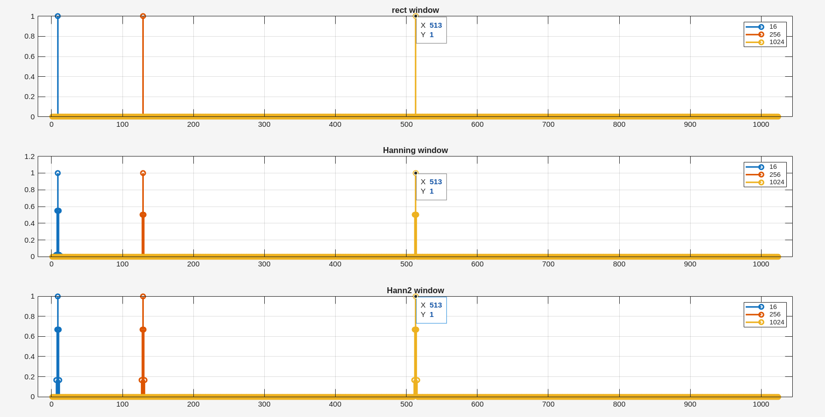
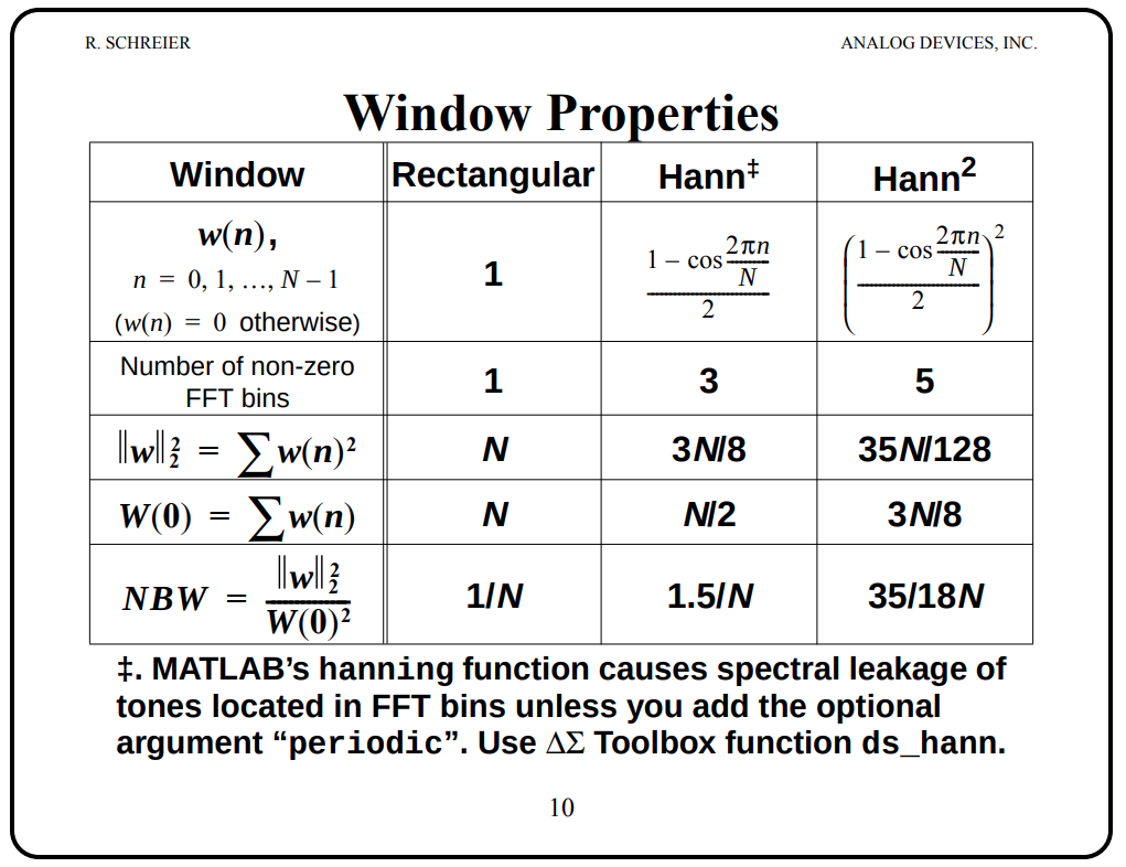
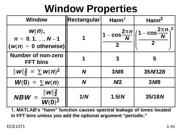
Nonzero FFT bins
everynanocounts. Memos on FFT With Windowing. [https://a2d2ic.wordpress.com/2018/02/01/memos-on-fft-with-windowing]
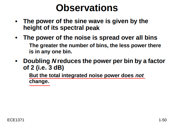
The problem with sine-wave scaling is that the noise power is, on average, evenly distributed over all FFT bins, whereas the sine-wave power is concentrated in only a few bins. With sine-wave scaling, the power of individual sine-wave components can be read directly from the spectral plot, but in order to determine the noise power, the powers of all the noise bins must be added together.

We can't use Fourier transform of random signal
[https://raytroop.github.io/2023/11/10/random/#lti-systems-on-wss-processes]
\[ \mathrm{SNR} = \frac{X_\text{sig}^2}{X_\text{n}^2N} = \frac{X_\text{sig}^2\cdot \sum_k W_k^2}{X_\text{n}^2N\cdot \sum_k W_k^2} = \frac{\sum_\text{nb} X_\text{w,sig}^2}{N X_\text{w,n}^2} \] where \(\text{nb}\) is number of non-zero FFT bins
1 | subplot(3,1,1); |
where \(\mathrm{NBW} = \frac{\sum_{n}|w[n]|^2}{ \left| \sum_{n} w[n] \right|^2}\)
1 | % excerpt of A.4 An Example in Pavan, Schreier and Temes, "Understanding Delta-Sigma Data Converters, Second Edition" ISBN 978-1-119-25827-8 |
Noise Floor
[http://individual.utoronto.ca/schreier/lectures/2015/1.pdf]
General Formula
signal tone power \[ P_{\text{sig}} = 2 \frac{X_{w,sig}^2}{S_1^2} \]
noise power \[ P_n = \frac{X_{w,n}^2}{N\cdot S_2}N=\frac{X_{w,n}^2}{S_2} \]
where white noise, \(X_n(i) = X_n(j)\) for any \(i \neq j\)
Therefore, displayed SNR is obtained \[\begin{align} \mathrm{SNR} &= 10\log10\left(\frac{X_{w,sig}^2}{X_{w,n}^2}\right) \\ &= 10\log_{10}\left(\frac{P_{\text{sig}}}{P_n}\right) + 10\log_{10}\left(\frac{S_1^2}{2S_2}\right) \\ &= \mathrm{SNR}'-10\log_{10}\left(\frac{2S_2}{S_1^2}\right) \\ &= \mathrm{SNR}'-10\log_{10}(2\cdot\mathrm{NBW}) \end{align}\]
DFT's output \(\mathrm{SNR}\)
\[ \text{PS(k)} = \text{PSD(k)} \cdot \text{ENBW} \]
where Effective Noise BandWidth \(\text{ENBW} =f_{\text{res}} \cdot \frac{N S_2}{S_1^2}\)
yield \[ \text{PS(k)} = \text{PSD(k)} \cdot f_{\text{res}} \cdot \frac{N S_2}{S_1^2} = \left\{\text{PSD(k)} \cdot f_{\text{s}} \right\} \cdot \frac{S_2}{S_1^2} \] where \(\left\{\text{PSD(k)} \cdot f_{\text{s}} \right\} =\text{const}\), i.e. \(x_\text{n,rms}\)
1 | ratio_list = []; |
FFT Noise Floor
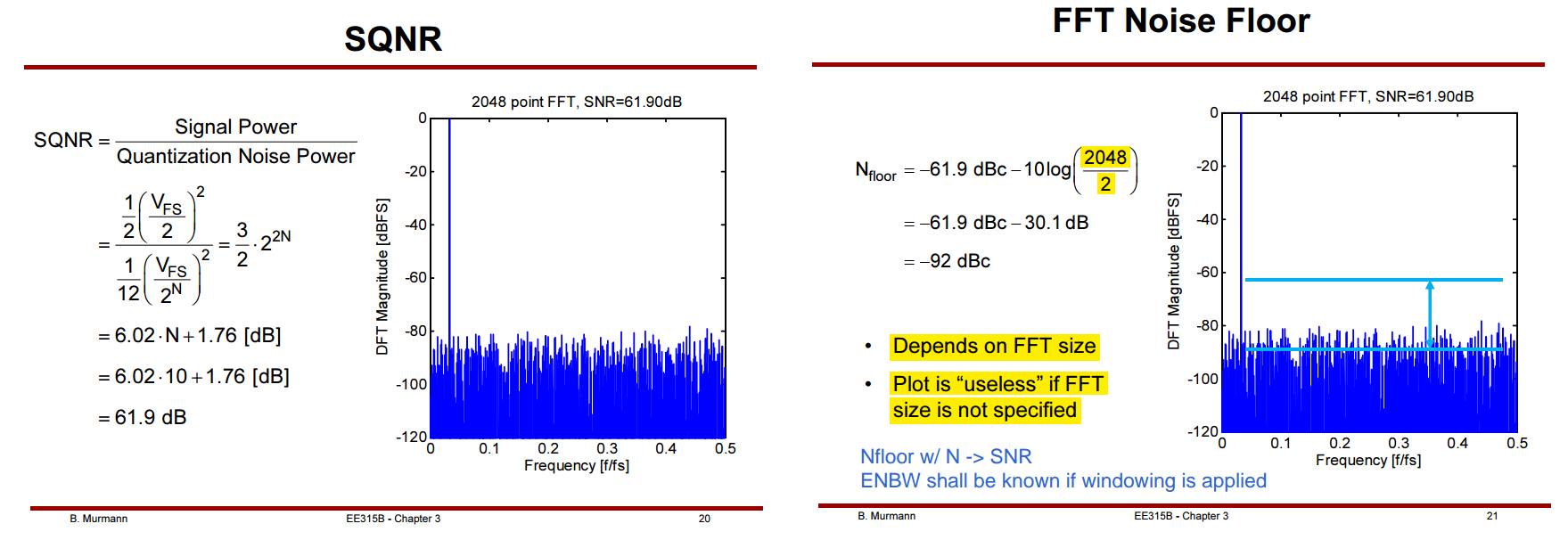
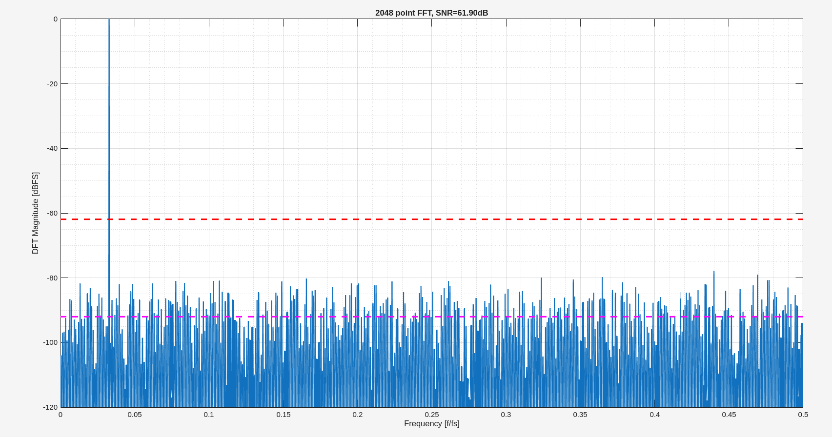
1 | N = 2048; |
Rectangular Window
DFT bin's output noise standard deviation (rms) value is proportional to \(\sqrt{N}\), and the DFT's output magnitude for the bin containing the signal tone is proportional to \(N\)
signal tone power \[ P_{\text{sig}} = 2 \frac{X_{w,sig}^2}{N^2} \]
noise power \[ P_n = \frac{X_{w,n}^2}{N} \]
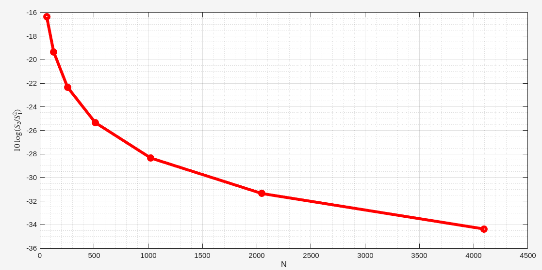
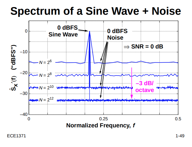
The displayed SNR \[ \mathrm{SNR} = \mathrm{SNR}' - 10\log_{10}(2/N) \] If we increase a DFT's size from \(N\) to \(2N\), the DFT's output SNR increased by 3dB. So we say that a DFT's processing gain increases by 3dB whenever \(N\) is doubled.
1 | for N=[2^6 2^8 2^10 2^12] |
output:
1 | -15.0515 |
How spectrum analyzer work?
We tried to plot a power spectral density together with something that we want to interpret as a power spectrum
- spectrum of a periodic signal
- spectral density of a broadband signal such as noise
Sine-wave components are located in individual FFT bins, but broadband signals like noise have their power spread over all FFT bins!
The noise floor depends on the length of the FFT
PS and PSD
The spectral density format is appropriate for random or noise signals but inappropriate for discrete frequency components because the latter theoretically have zero bandwidth
Amplitude Correction
A finite-duration window \(w[n]\)
DTFT is \(W[e^{j\omega}]\) and the maximum magnitude is is at DC frequency, which \(\sum_n w_n\)
Sinusoidal signal \(x[n]\)
DFS is \(X_k\), and DTFT shall be \(\frac{2\pi}{N}X_k(e^{j\omega})\)
the windowed sequence \(v[n] = x[n]w[n]\)
with multiplication property, DTFT of \(v[n]\) shall be \(\frac{X_k(e^{j\omega})}{N}\sum_n w_n\)
As we know, DFT of \(v[n]\) is samples of its DTFT, that is \[ \frac{X_k(e^{j\omega})}{N}\sum_n w_n = X_v[k] \] Therefore, \[ \frac{X_k(e^{j\omega})}{N} = \frac{X_v[k]}{\sum_n w_n} \]
Effective Noise BandWidth (ENBW)
General derivation
The relationship between a power spectrum (\(PS, V^2\)) and a power spectral density (\(PSD, V^2/Hz\)) is given by the effective noise bandwidth (ENBW), which can easily be determined at the time when the DFT is computed.
ENBW should always be recorded when a spectrum or spectral density is computed, such that the result can be converted to the other form at a later stage, when the information about the frequency resolution \(f_{res}\) and the window that was used is normally not easily available any more.
The normalized equivalent noise bandwidth (NENBW) of the window is given by
\[ \text{NENBW} = \frac{NS_2}{S_1^2} \] where \(S_1 = \sum _{k=0}^{N-1}w_k\) and \(S_2 = \sum _{k=0}^{N-1}w_k^2\)
The ENBW is given by
\[ \text{ENBW} = \text{NENBW}\cdot f_{res} = \text{NENBW}\cdot \frac{f_s}{N} = f_s\frac{S_2}{S_1^2} \]
Equivalent noise bandwidth (ENBW) compares a window to an ideal, rectangular time-window. It is the bandwidth of the rectangular window's frequency-domain shape that passes the same amount of white noise energy as the frequency-domain shape defined by the other window.
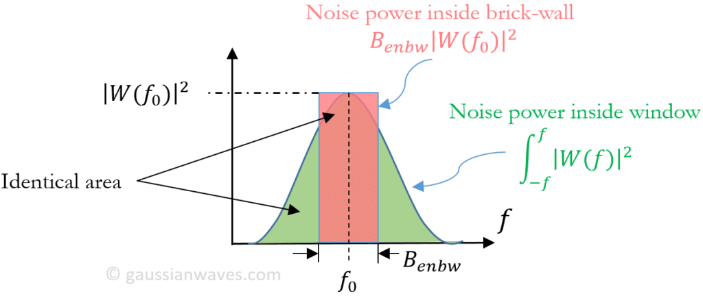
Therefore, the equivalent noise bandwidth \(B_{enbw}\) is given by
\[ B_{enbw} = \frac{\int_{-f}^{f} |W(f)|^2 df}{|W(f_0)|^2} \]
Translating to discrete domain, the equivalent noise bandwidth can be computed using DFT samples as
\[ B_{enbw} =\frac{\sum_{k=0}^{N-1}|W[k]|^2}{|W[k_0]|^2} \]
where \(k_0\) is the index at which the magnitude of FFT output is maximum and \(N\) is the window length, i.e. \(k_0=0\).
Applying Parseval's theorem and \(W[0]=\sum_{n}w[n]\), \(B_{enbw}\) can also be computed using time domain samples as
\[ B_{enbw} = N \frac{\sum_{n}|w[n]|^2}{ \left| \sum_{n} w[n] \right|^2} \]
scale \(w[n]\) don't change \(B_{enbw}\)
Noise power inside window: \(\int_{-f}^{f} |W(f)|^2 df \to N\cdot\sum_{n}|w[n]|^2\)
peak amplitude: \(|W(f_0)|^2 \to \left| \sum_{n} w[n] \right|^2\)
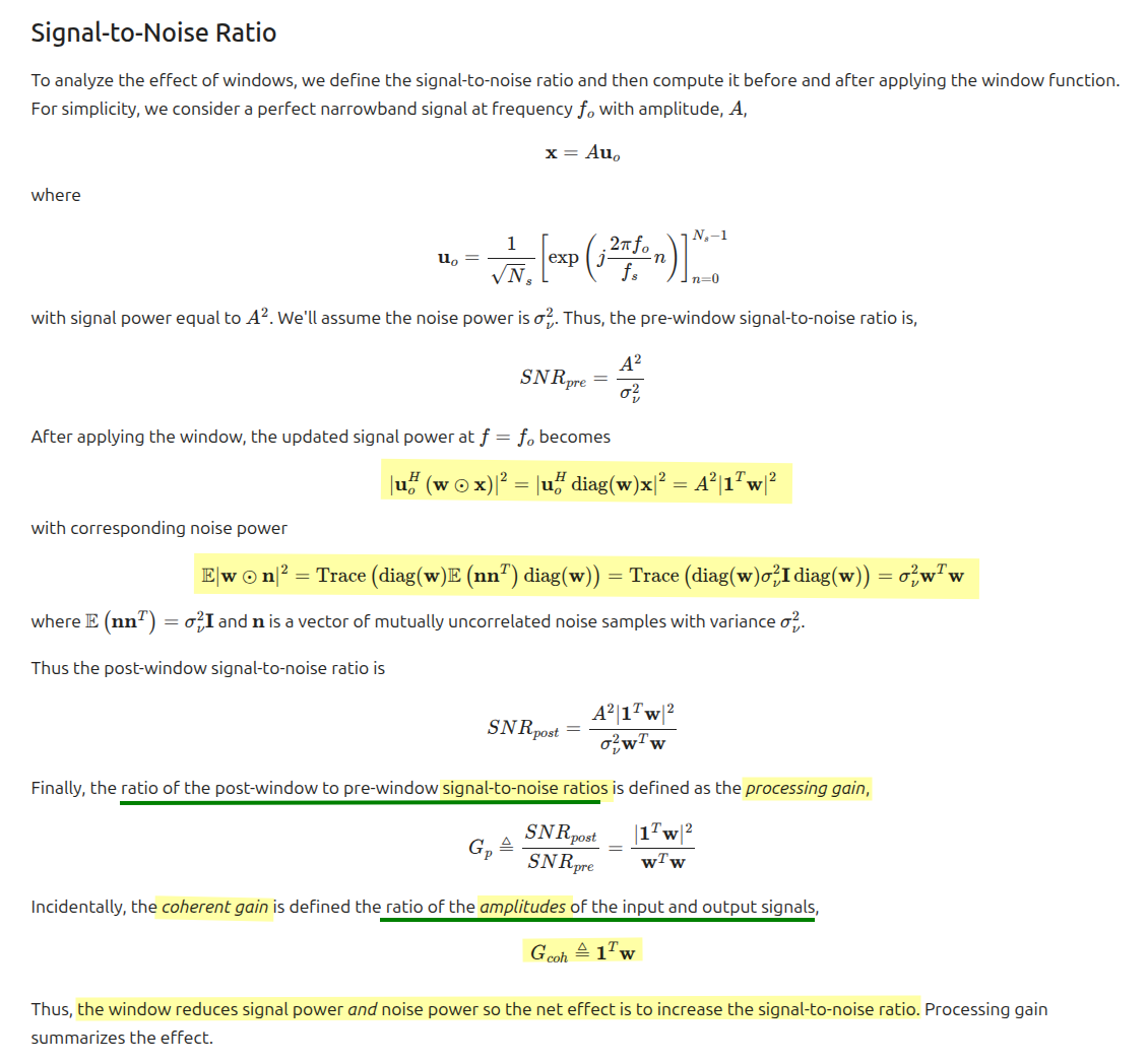
An alternative derivation

Assuming the windowed sequence \(v[n] = x[n]w[n]\)
\(W[k]\): Fourier Transform of finite sequence window
\(X_{sig}\): Fourier Transform of signal
\(X_{n}\): Fourier Transform of noise
\(X_{v,sig}\): Fourier Transform of windowed signal
\(X_{v,n}\): Fourier Transform of windowed noise
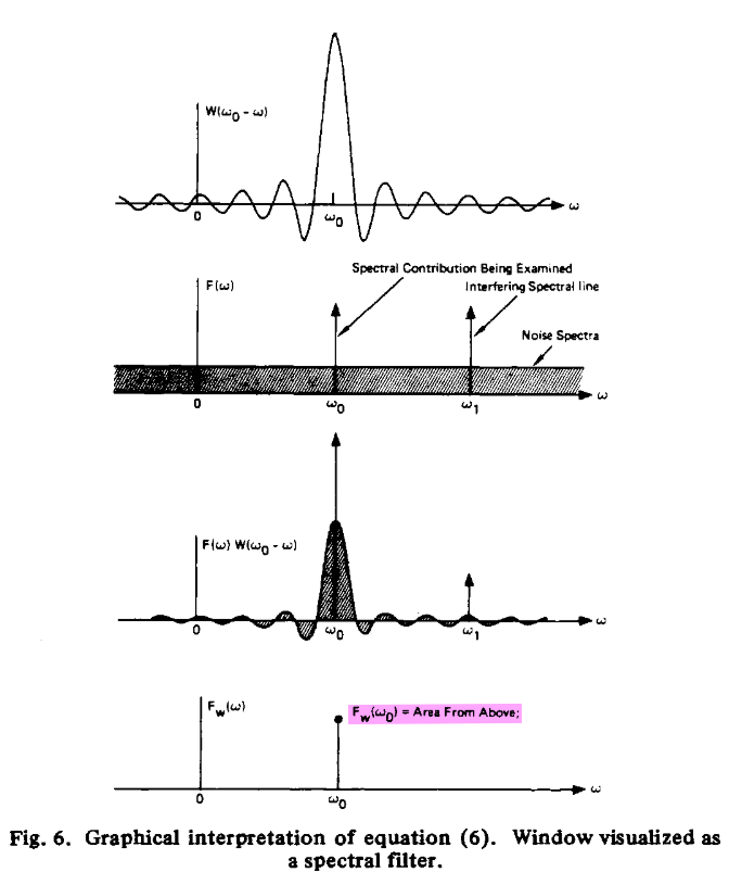
From Fig. 6,, we observe that the amplitude of the harmonic estimate at a given frequency is biased by the accumulated broad-band noise included in the bandwidth of the window.
In this sense, the window behaves as a filter, gathering contributions for its estimate over its bandwidth
The Fourier Transform of windowed signal can be expressed as
\[\begin{align} X_{v,sig} &= W_{max}\cdot X_{sig} \\ &= W[0]\cdot X_{sig} \end{align}\]
For a typical window, \(W_{max}\) occurs at \(\omega = 0\)
And the Fourier Transform of windowed noise can be expressed as
\[ X_{v,n}^2 = \sum_k (W[k])^2 \cdot X_n^2 \]
divided by \((W[0])^2\) on both sides of the above equation
\[ \frac{X_{v,n}^2}{(W[0])^2} = \frac{\sum_k (W[k])^2}{(W[0])^2} \cdot X_n^2 \]
By Parseval's theorem
\[ \frac{X_{v,n}^2}{\left(\sum_n w[n]\right)^2} = \frac{N\sum_n w^2[n]}{\left(\sum_n w[n]\right)^2} \cdot X_n^2 \]
where \(X^2_n\) is what is deserved and
\[ X_n^2 = \frac{PS_{n}}{B_{enbw}} \]
where \(B_{enbw} = N \frac{\sum_{n}|w[n]|^2}{ \left| \sum_{n} w[n] \right|^2}\) and \(PS_{n}=\left| \frac{X_{v,n}}{\sum_n w[n]}\right|^2\)
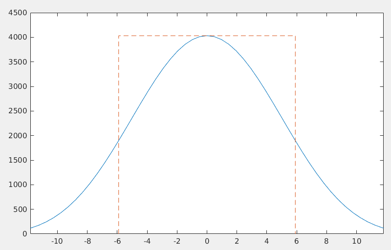
example
1 | lw = 128; |
Verify that the area of the rectangle contains the same total power
as the window. 1
Adiff = trapz(freq,ad)-bw*mg
1
2
3
bw: 11.811
bdef: 11.811
Adiff: 7.276e-12
Unpingco, José. Python for Signal Processing: Featuring IPython Notebooks. Cham: Springer, 2013. [pdf]
[https://github.com/unpingco/Python-for-Signal-Processing/blob/master/Windowing_Part2.ipynb]
demo
1 | %https://aaronscher.com/Course_materials/Communication_Systems/documents/PSD_Autocorrelation_Noise.pdf |

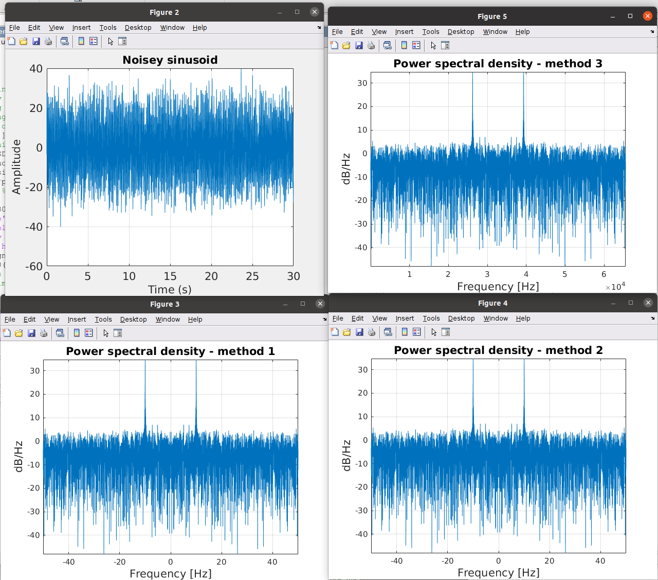
The power spectral density plots for methods 2 and 3 exactly match that for method 1 (shown above).
reference
enbw Matlab URL:https://www.mathworks.com/help/signal/ref/enbw.html
1 | N = 256; |
1 | ans = |
Schmid, H. (2012). How to use the FFT and Matlab's pwelch function for signal and noise simulations and measurements. URL:http://www.schmid-werren.ch/hanspeter/publications/2012fftnoise.pdf
Bonnie C.Baker. Reading and Using Fast Fourier Transforms (FFT) URL:http://ww1.microchip.com/downloads/en/appnotes/00681a.pdf
FFT analysis: SNR and Noise level vary with FFT Window size URL:https://www.virtins.com/forum/viewtopic.php?f=7&t=1382
Lyons, R. G. (2011). Understanding digital signal processing (3rd ed.). Prentice Hall
Stefan Scholl, "Exact Signal Measurements using FFT Analysis",Microelectronic Systems Design Research Group, TU Kaiserslautern, Germany. [pdf]
Aaron Scher. PSD, Autocorrelation, and Noise in MATLAB [pdf]
Aaron Scher. FFT, total energy, and energy spectral density computations in MATLAB [pdf]
Amplitude Estimation and Zero Padding URL:https://www.mathworks.com/help/signal/ug/amplitude-estimation-and-zero-padding.html
Harris, F. (1978). On the use of windows for harmonic analysis with the discrete Fourier transform. Proceedings of the IEEE, 66, 51-83. [pdf]
Harris, F. J. . (1976). Windows, harmonic analysis and the discrete fourier transform. [pdf]
Wang Hongwei. Virtins. Evaluation of Various Window Functions using Multi-Instrument [pdf]
Properties of FFT Windows Used in Stable32 [pdf]
Solomon, Jr, O M. PSD computations using Welch's method. [Power Spectral Density (PSD)]. United States. https://doi.org/10.2172/5688766 [pdf]
Measure Power of Deterministic Periodic Signals [https://www.mathworks.com/help/signal/ug/measuring-the-power-of-deterministic-periodic-signals.html]
Mathuranathan. Equivalent noise bandwidth (ENBW) of window functions. [https://www.gaussianwaves.com/2020/09/equivalent-noise-bandwidth-enbw-of-window-functions/]
recordingblogs, Equivalent noise bandwidth [https://www.recordingblogs.com/wiki/equivalent-noise-bandwidth]
unpingco, Python for Signal Processing [https://github.com/unpingco/Python-for-Signal-Processing/blob/master/Windowing_Part2.ipynb]
Pavan, Schreier and Temes, "Understanding Delta-Sigma Data Converters, Second Edition" ISBN 978-1-119-25827-8