Periodic Analysis
PSS and HB Overview
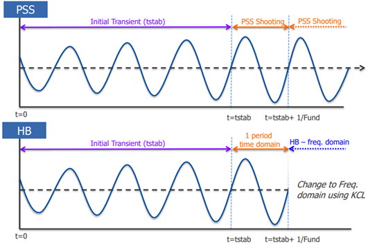
The steady-state response is the response that results after any transient effects have dissipated.
The large signal solution is the starting point for small-signal analyses, including periodic AC, periodic transfer function, periodic noise, periodic stability, and periodic scattering parameter analyses.
Designers refer periodic steady state analysis in time domain as "PSS" and corresponding frequency domain notation as "HB"
Harmonic Balance Analysis
The idea of harmonic balance is to find a set of port voltage waveforms (or, alternatively, the harmonic voltage components) that give the same currents in both the linear-network equations and nonlinear-network equations
that is, the currents satisfy Kirchoff's current law
Define an error function at each harmonic, \(f_k\), where \[ f_k = I_{\text{LIN}}(k\omega) + I_{\text{NL}}(k\omega) \] where \(k=0, 1, 2,...,K\)
Note that each \(f_k\) is implicitly a function of all voltage components \(V(k\omega)\)
Newton Solution of the Harmonic-Balance Equation
Iterative Process and Jacobian Formulation
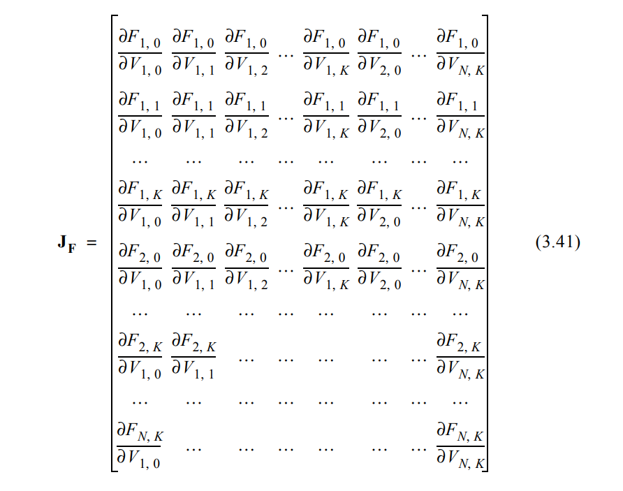
The elements of the Jacobian are the derivatives \[ \frac{\partial F_{\text{n,k}}}{\partial _{V_\text{m,l}}} \] where \(n\) and \(m\) are the port indices \((1,N)\), and \(k\) and \(l\) are the harmonic indices \((0,...,K)\)
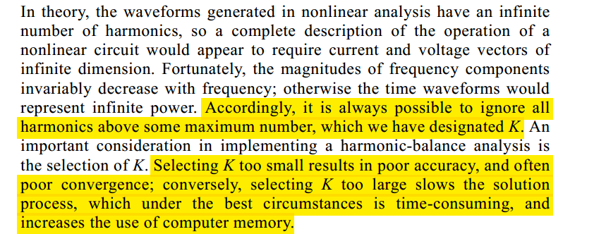
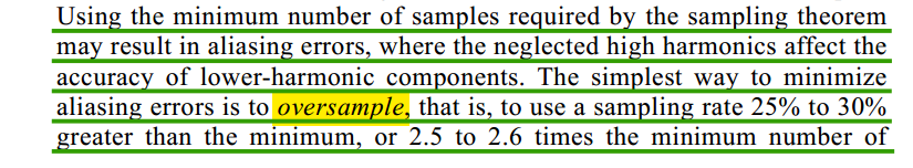
Number of Harmonics & Time Samples
Initial Estimate
One important property of Newton's method is that its speed and reliability of convergence depend strongly upon the initial estimate of the solution vector.
Conversion Matrix Analysis
Large-signal/small-signal analysis, or conversion matrix analysis, is useful for a large class of problems wherein a nonlinear device is driven, or "pumped" by a single large sinusoidal signal; another signal, much smaller, is applied; and we seek only the linear response to the small signal.
The most common application of this technique is in the design of mixers and in nonlinear noise analysis
- First, analyzing the nonlinear device under large-signal excitation only, where the harmonic-balance method can be applied
- Then, the nonlinear elements in the device's equivalent circuit are then linearized to create small-signal, linear, time-varying elements
- Finally, a small-signal analysis is performed
Element Linearized
Below shows a nonlinear resistive element, which has the \(I/V\) relationship \(I=f(V)\). It is driven by a large-signal voltage
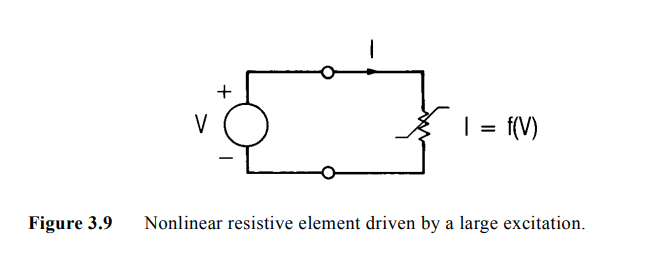
Assuming that \(V\) consists of the sum of a large-signal component \(V_0\) and a small-signal component \(v\), with Taylor series \[ f(V_0+v) = f(V_0)+\frac{d}{dV}f(V)|_{V=V_0}\cdot v+\frac{1}{2}\frac{d^2}{dV^2}f(V)|_{V=V_0}\cdot v^2+... \] The small-signal, incremental current is found by subtracting the large-signal component of the current \[ i(v)=I(V_0+v)-I(V_0) \] If \(v \ll V_0\), \(v^2\), \(v^3\),... are negligible. Then, \[ i(v) = \frac{d}{dV}f(V)|_{V=V_0}\cdot v \]
\(V_0\) need not be a DC quantity; it can be a time-varying large-signal voltage \(V_L(t)\) and that \(v=v(t)\), a function of time. Then \[ i(t)=g(t)v(t) \] where \(g(t)=\frac{d}{dV}f(V)|_{V=V_L(t)}\)
The time-varying conductance \(g(t)\), is the derivative of the element's \(I/V\) characteristic at the large-signal voltage
By an analogous derivation, one could have a current-controlled resistor with the \(V/I\) characteristic \(V = f_R(I)\) and obtain the small-signal \(v/i\) relation \[ v(t) = r(t)i(t) \] where \(r(t) = \frac{d}{dI}f_R(I)|_{I=I_L(t)}\)
A nonlinear element excited by two tones supports currents and voltages at mixing frequencies \(m\omega_1+n\omega_2\), where \(m\) and \(n\) are integers. If one of those tones, \(\omega_1\) has such a low level that it does not generate harmonics and the other is a large-signal sinusoid at \(\omega_p\), then the mixing frequencies are \(\omega=\pm\omega_1+n\omega_p\), which shown in below figure
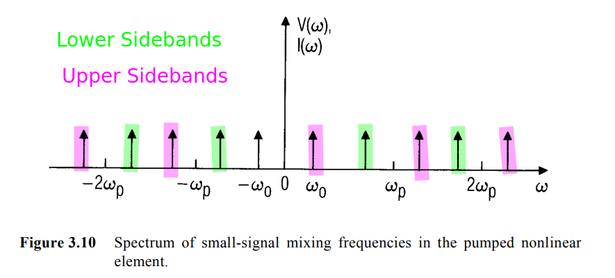
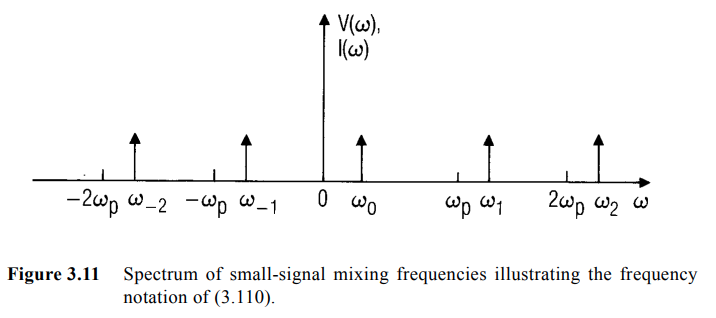
A more compact representation of the mixing frequencies is \[ \omega_n=\omega_0+n\omega_p \] which includes only half of the mixing frequencies:
- the negative components of the lower sidebands (LSB)
- and the positive components of the upper sidebands (USB)
For real signal, positive- and negative-frequency components are complex conjugate pairs
Shooting Newton
TODO 📅
Nonlinearity & Linear Time-Varying Nature
Nonlinearity Nature
The nonlinearity causes the signal to be replicated at multiples of the carrier, an effect referred to as harmonic distortion, and adds a skirt to the signal that increases its bandwidth, an effect referred to as intermodulation distortion
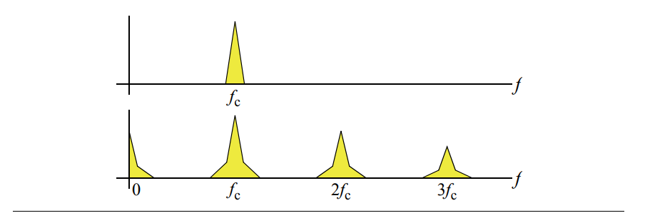
It is possible to eliminate the effect of harmonic distortion with a bandpass filter, however the frequency of the intermodulation distortion products overlaps the frequency of the desired signal, and so cannot be completely removed with filtering.
Time-Varying Linear Nature
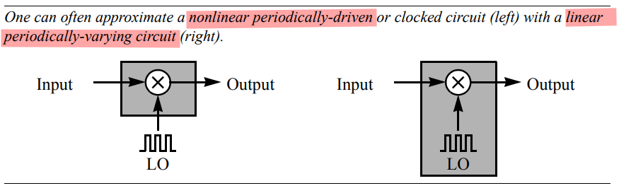
linear with respect to \(v_{in}\) and time-varying
Given \(v_{in}(t)=m(t)\cos (\omega_c t)\) and LO signal of \(\cos(\omega_{LO} t)\), then \[ v_{out}(t) = \text{LPF}\{m(t)\cos(\omega_c t)\cdot \cos(\omega_{LO} t)\} \] and \[ v_{out}(t) = m(t)\cos((\omega_c - \omega_{LO})t) \]
A linear periodically-varying transfer function implements frequency translation
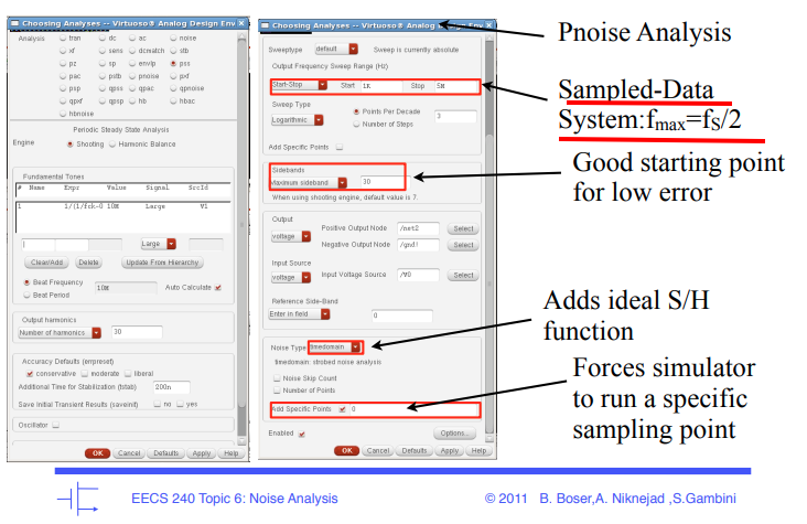
Periodic small signal analyses
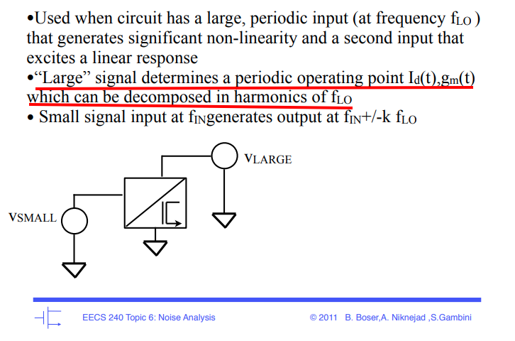
Analysis in Simulator
- LPV analyses start by performing a periodic analysis to compute the periodic operating point with only the large clock signal applied (the LO, the clock, the carrier, etc.).
- The circuit is then linearized about this time-varying operating point (expand about the periodic equilibrium point with a Taylor series and discard all but the first-order term)
- and the small information signal is applied. The response is calculated using linear time-varying analysis
Versions of this type of small-signal analysis exists for both harmonic balance and shooting methods
PAC is useful for predicting the output sidebands produced by a particular input signal
PXF is best at predicting the input images for a particular output
Linear Time Varying
The response of a relaxed LTV system at a time \(t\) due to an impulse applied at a time \(t − \tau\) is denoted by \(h(t, \tau)\)
The first argument in the impulse response denotes the time of observation.
The second argument indicates that the system was excited by an impulse launched at a time \(\tau\) prior to the time of observation.
Thus, the response of an LTV system not only depends on how long before the observation time it was excited by the impulse but also on the observation instant.
The output \(y(t)\) of an initially relaxed LTV system with impulse response \(h(t, \tau)\) is given by the convolution integral \[ y(t) = \int_0^{\infty}h(t,\tau)x(t-\tau)d\tau \] Assuming \(x(t) = e^{j2\pi f t}\) \[ y(t) = \int_0^{\infty}h(t,\tau)e^{j2\pi f (t-\tau)}d\tau = e^{j2\pi f t}\int_0^{\infty}h(t,\tau)e^{-j2\pi f\tau}d\tau \] The (time-varying) frequency response can be interpreted as \[ H(j2\pi f, t) = \int_0^{\infty}h(t,\tau)e^{-j2\pi f\tau}d\tau \] Linear Periodically Time-Varying (LPTV) Systems, which is a special case of an LTV system whose impulse response satisfies \[ h(t, \tau) = h(t+T_s, \tau) \] In other words, the response to an impulse remains unchanged if the time at which the output is observed (\(t\)) and the time at which the impulse is applied (denoted by \(t_1\)) are both shifted by \(T_s\) \[ H(j2\pi f, t+T_s) = \int_0^{\infty}h(t+T_s,\tau)e^{-j2\pi f\tau}d\tau = \int_0^{\infty}h(t,\tau)e^{-j2\pi f\tau}d\tau = H(j2\pi f, t) \] \(H(j2\pi f, t)\) of an LPTV system is periodic with timeperiod \(T_s\), it can be expanded as a Fourier series in \(t\), resulting in \[ H(j2\pi f, t) = \sum_{k=-\infty}^{\infty} H_k(j2\pi f)e^{j2\pi f_s k t} \] The coefficients of the Fourier series \(H_k(j2\pi f)\) are given by \[ H_k(j2\pi f) = \frac{1}{T_s}\int_0^{T_s} H(j2\pi f, t) e^{-j2\pi k f_s t}dt \]
reference
K. S. Kundert, "Introduction to RF simulation and its application," in IEEE Journal of Solid-State Circuits, vol. 34, no. 9, pp. 1298-1319, Sept. 1999, doi: 10.1109/4.782091. [pdf]
Stephen Maas, Nonlinear Microwave and RF Circuits, Second Edition , Artech, 2003. [pdf]
Karti Mayaram. ECE 521 Fall 2016 Analog Circuit Simulation: Simulation of Radio Frequency Integrated Circuits [pdf1, pdf2]
The Value Of RF Harmonic Balance Analyses For Analog Verification: Frequency domain periodic large and small signal analyses. [https://semiengineering.com/the-value-of-rf-harmonic-balance-analyses-for-analog-verification/]
Shanthi Pavan, "Demystifying Linear Time Varying Circuits"
S. Pavan and G. C. Temes, "Reciprocity and Inter-Reciprocity: A Tutorial— Part I: Linear Time-Invariant Networks," in IEEE Transactions on Circuits and Systems I: Regular Papers, vol. 70, no. 9, pp. 3413-3421, Sept. 2023, doi: 10.1109/TCSI.2023.3276700.
S. Pavan and G. C. Temes, "Reciprocity and Inter-Reciprocity: A Tutorial—Part II: Linear Periodically Time-Varying Networks," in IEEE Transactions on Circuits and Systems I: Regular Papers, vol. 70, no. 9, pp. 3422-3435, Sept. 2023, doi: 10.1109/TCSI.2023.3294298.
S. Pavan and R. S. Rajan, "Interreciprocity in Linear Periodically Time-Varying Networks With Sampled Outputs," in IEEE Transactions on Circuits and Systems II: Express Briefs, vol. 61, no. 9, pp. 686-690, Sept. 2014, doi: 10.1109/TCSII.2014.2335393.
Prof. Shanthi Pavan. Introduction to Time - Varying Electrical Network. [https://youtube.com/playlist?list=PLyqSpQzTE6M8qllAtp9TTODxNfaoxRLp9]
Shanthi Pavan. EE5323: Advanced Electrical Networks (Jan-May. 2015) [https://www.ee.iitm.ac.in/vlsi/courses/ee5323/start]
R. S. Ashwin Kumar. EE698W: Analog circuits for signal processing [https://home.iitk.ac.in/~ashwinrs/2022_EE698W.html]
Piet Vanassche, Georges Gielen, and Willy Sansen. 2009. Systematic Modeling and Analysis of Telecom Frontends and their Building Blocks (1st. ed.). Springer Publishing Company, Incorporated.
Beffa, Federico. (2023). Weakly Nonlinear Systems. 10.1007/978-3-031-40681-2.
Wereley, Norman. (1990). Analysis and control of linear periodically time varying systems.
Hameed, S. (2017). Design and Analysis of Programmable Receiver Front-Ends Based on LPTV Circuits. UCLA. ProQuest ID: Hameed_ucla_0031D_15577. Merritt ID: ark:/13030/m5gb6zcz. Retrieved from https://escholarship.org/uc/item/51q2m7bx
Matt Allen. Introduction to Linear Time Periodic Systems. [https://youtu.be/OCOkEFDQKTI]
Fivel, Oren. "Analysis of Linear Time-Varying & Periodic Systems." arXiv preprint arXiv:2202.00498 (2022).
RF Harmonic Balance Analysis for Nonlinear Circuits [https://resources.pcb.cadence.com/blog/2019-rf-harmonic-balance-analysis-for-nonlinear-circuits]
Steer, Michael. Microwave and RF Design (Third Edition, 2019). NC State University, 2019.
Steer, Michael. Harmonic Balance Analysis of Nonlinear RF Circuits - Case Study Index: CS_AmpHB [link]
Vishal Saxena, "SpectreRF Periodic Analysis" URL:https://www.eecis.udel.edu/~vsaxena/courses/ece614/Handouts/SpectreRF%20Periodic%20Analysis.pdf
Josh Carnes,Peter Kurahashi. "Periodic Analyses of Sampled Systems" URL:https://slideplayer.com/slide/14865977/
Kundert, Ken. (2006). Simulating Switched-Capacitor Filters with SpectreRF. URL:https://designers-guide.org/analysis/sc-filters.pdf
Article (20482538) Title: Why is pnoise sampled(jitter) different than pnoise timeaverage on a driven circuit?
Article (20467468) Title: The mathematics behind choosing the upper frequency when simulating pnoise jitter on an oscillator
Andrew Beckett. "Simulating phase noise for PFD-CP". URL:https://groups.google.com/g/comp.cad.cadence/c/NPisXTElx6E/m/XjWxKbbfh2cJ
Dr. Yanghong Huang. MATH44041/64041: Applied Dynamical Systems [https://personalpages.manchester.ac.uk/staff/yanghong.huang/teaching/MATH4041/default.htm]
Jeffrey Wong. Math 563, Spring 2020 Applied computational analysis [https://services.math.duke.edu/~jtwong/math563-2020/main.html]
Jeffrey Wong. Math 353, Fall 2020 Ordinary and Partial Differential Equations [https://services.math.duke.edu/~jtwong/math353-2020/main.html]
Tip of the Week: Please explain in more practical (less theoretical) terms the concept of "oscillator line width." [https://community.cadence.com/cadence_blogs_8/b/rf/posts/please-explain-in-more-practical-less-theoretical-terms-the-concept-of-quot-oscillator-line-width-quot]
Rubiola, E. (2008). Phase Noise and Frequency Stability in Oscillators (The Cambridge RF and Microwave Engineering Series). Cambridge: Cambridge University Press. doi:10.1017/CBO9780511812798
Dr. Ulrich L. Rohde, Noise Analysis, Then and Today [https://www.microwavejournal.com/articles/29151-noise-analysis-then-and-today]
Nicola Da Dalt and Ali Sheikholeslami. 2018. Understanding Jitter and Phase Noise: A Circuits and Systems Perspective (1st. ed.). Cambridge University Press, USA.
Kester, Walt. (2005). Converting Oscillator Phase Noise to Time Jitter. [https://www.analog.com/media/en/training-seminars/tutorials/MT-008.pdf]
Drakhlis, B.. (2001). Calculate oscillator jitter by using phase-noise analysis: Part 2 of two parts. Microwaves and Rf. 40. 109-119.
Explanation for sampled PXF analysis. [https://community.cadence.com/cadence_technology_forums/f/custom-ic-design/45055/explanation-for-sampled-pxf-analysis/1376140#1376140]
模拟放大器的低噪声设计技术2-3实践 아날로그 증폭기의 저잡음 설계 기법2-3실습 [https://youtu.be/vXLDfEWR31k]
2.2 How POP Really Works [https://www.simplistechnologies.com/documentation/simplis/ast_02/topics/2_2_how_pop_really_works.htm]
Jaeha Kim. Lecture 11. Mismatch Simulation using PNOISE [https://ocw.snu.ac.kr/sites/default/files/NOTE/7037.pdf]
Hueber, G., & Staszewski, R. B. (Eds.) (2010). Multi-Mode/Multi-Band RF Transceivers for Wireless Communications: Advanced Techniques, Architectures, and Trends. John Wiley & Sons. https://doi.org/10.1002/9780470634455
B. Boser,A. Niknejad ,S.Gambin 2011 EECS 240 Topic 6: Noise Analysis [https://mixsignal.files.wordpress.com/2013/06/t06noiseanalysis_simone-1.pdf]