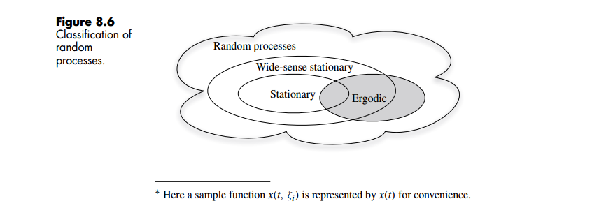
Random Process
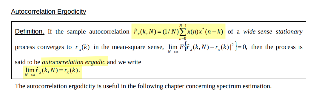
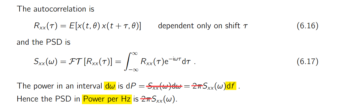
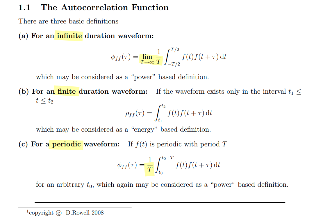
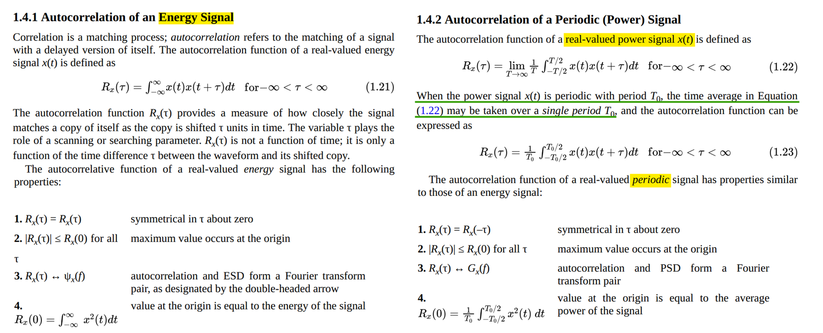
autocorrelation
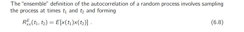
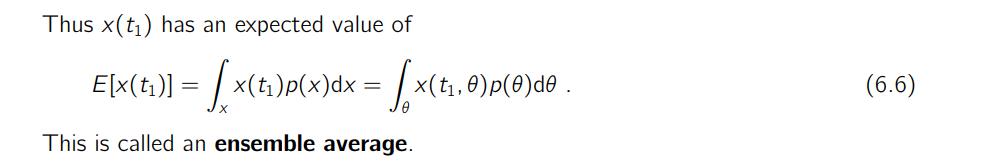
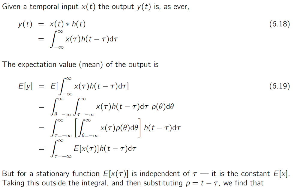
The expectation returns the probability-weighted average of the specific function at that specific time over all possible realizations of the process
Derivatives of Random Processes
since \(x(t)\) is stationary process, and \(y(t) = \frac{dx(t)}{dt}\)
Using \(R_{yy}(\tau) = h(\tau)*R_{xx}(\tau)*h(-\tau)\)
\[\begin{align} R_{yy}(\tau) &= \mathcal{F}^{-1}[H(j\omega)\Phi_{xx}(j\omega)H(-j\omega)] \\ &= \mathcal{F}^{-1}[-(j\omega)^2\Phi_{xx}(j\omega)] \end{align}\]
we obtain the autocorrelation function of the output process as \[ R_{yy}(\tau) = -\frac{d^2}{d\tau^2}R_{xx}(\tau) \]
Liu Congfeng, Xidian University. Random Signal Processing: Chapter 5 Linear System: Random Process [https://web.xidian.edu.cn/cfliu/files/20121125_153218.pdf]
[https://sharif.ir/~bahram/sp4cl/PapoulisLectureSlides/lectr14.pdf]
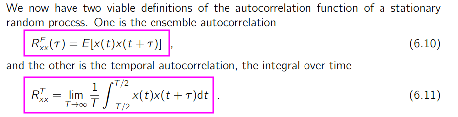
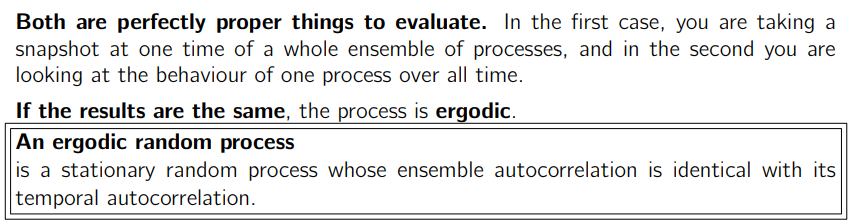
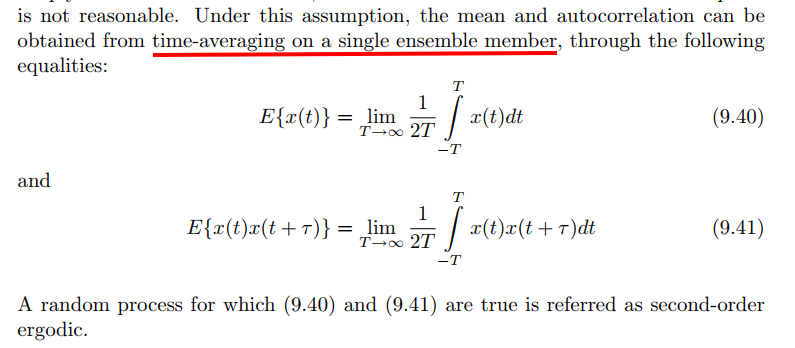
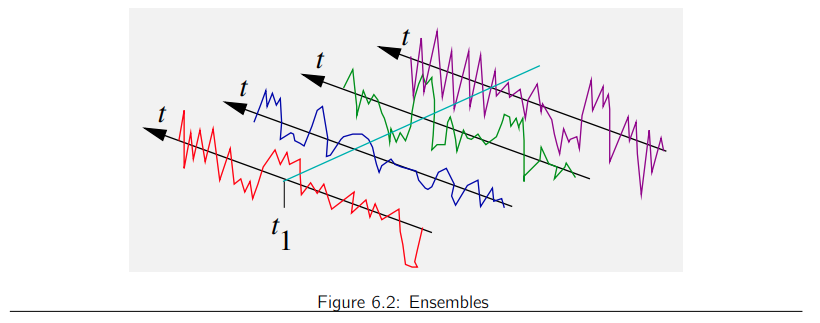
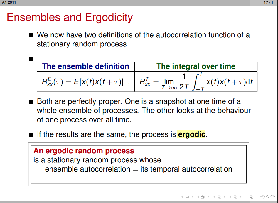
Ergodicity
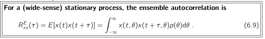
ensemble autocorrelation and temporal autocorrelation (time autocorrelation)
ECE438 - Laboratory 7: Discrete-Time Random Processes (Week 2) October 6, 2010 [https://engineering.purdue.edu/VISE/ee438L/lab7/pdf/lab7b.pdf]
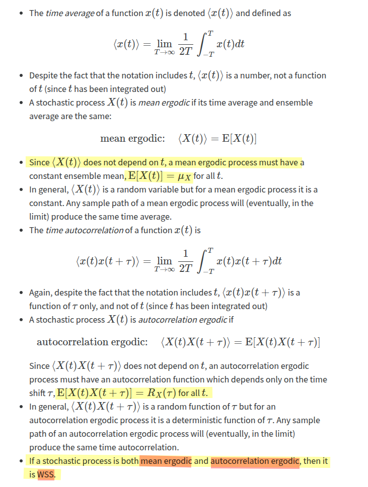
Ensemble Averages & Time Averages
[https://ece-research.unm.edu/bsanthan/ece541/stat.pdf]
[https://www.nii.ac.jp/qis/first-quantum/e/forStudents/lecture/pdf/noise/chapter1.pdf]
- time average: time-averaged quantities for the \(i\)-th member of the ensemble
- ensemble average: ensemble-averaged quantities for all members of the ensemble at a certain time
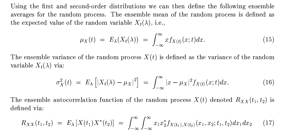
where \(\theta\) is one member of the ensemble; \(p(x)dx\) is the probability that \(x\) is found among \([x, x + dx]\)
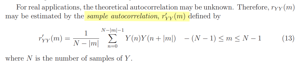
sample autocorrelation
[https://engineering.purdue.edu/VISE/ee438L/lab7/pdf/lab7b.pdf]
[http://www.signal.uu.se/Courses/CourseDirs/SignalbehandlingIT/forelas02.pdf]
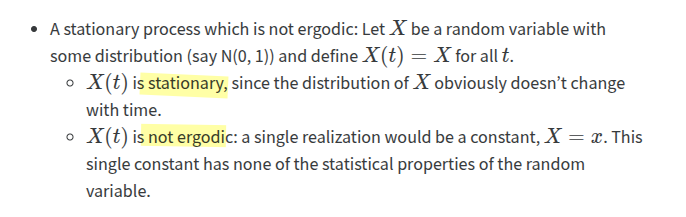
ergodic vs. stationary
[https://bookdown.org/kevin_davisross/stat350-handouts/stationary.html]
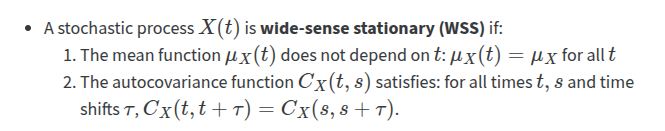
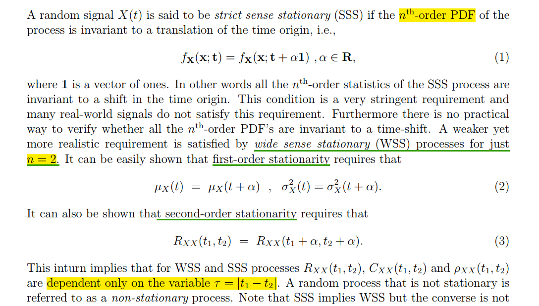
Strict Sense Stationary (SSS) & Wide Sense Stationary (WSS)
mean
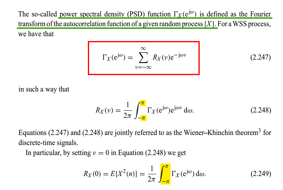
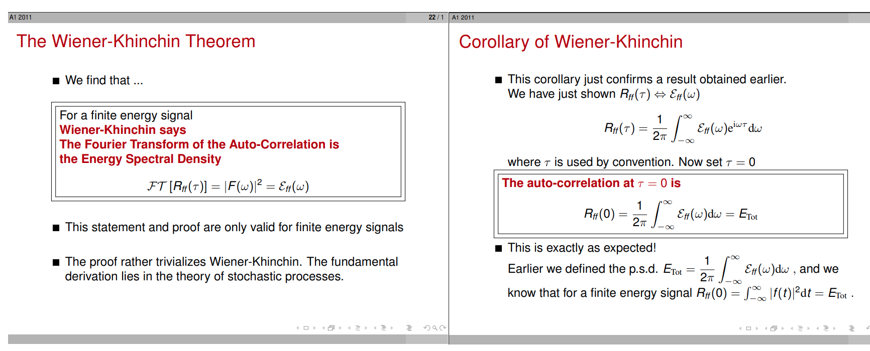
Wiener-Khinchin theorem
Norbert Wiener proved this theorem for the case of a deterministic function in 1930; Aleksandr Khinchin later formulated an analogous result for stationary stochastic processes and published that probabilistic analogue in 1934. Albert Einstein explained, without proofs, the idea in a brief two-page memo in 1914
Continuous time
[https://www.robots.ox.ac.uk/~dwm/Courses/2TF_2011/2TF-L5.pdf]
Frank R. Kschischang. The Wiener-Khinchin Theorem [https://www.comm.utoronto.ca/~frank/notes/wk.pdf]
\(x(t)\), Fourier transform over a limited period of time \([-T/2, +T/2]\) , \(X_T(f) = \int_{-T/2}^{T/2}x(t)e^{-j2\pi ft}dt\)
With Parseval's theorem \[ \int_{-T/2}^{T/2}|x(t)|^2dt = \int_{-\infty}^{\infty}|X_T(f)|^2df \] So that \[ \frac{1}{T}\int_{-T/2}^{T/2}|x(t)|^2dt = \int_{-\infty}^{\infty}\frac{1}{T}|X_T(f)|^2df \]
where the quantity, \(\frac{1}{T}|X_T(f)|^2\) can be interpreted as distribution of power in the frequency domain
For each \(f\) this quantity is a random variable, since it is a function of the random process \(x(t)\)
The power spectral density (PSD) \(S_x(f )\) is defined as the limit of the expectation of the expression above, for large \(T\): \[ S_x(f) = \lim _{T\to \infty}\mathrm{E}\left[ \frac{1}{T}|X_T(f)|^2 \right] \]
The Wiener-Khinchin theorem ensures that for well-behaved wide-sense stationary processes the limit exists and is equal to the Fourier transform of the autocorrelation \[\begin{align} S_x(f) &= \int_{-\infty}^{+\infty}R_x(\tau)e^{-j2\pi f \tau}d\tau \\ R_x(\tau) &= \int_{-\infty}^{+\infty}S_x(f)e^{j2\pi f \tau}df \end{align}\]
Note: \(S_x(f)\) in Hz and inverse Fourier Transform in Hz (\(\frac{1}{2\pi}d\omega = df\))
Topic 6 Random Processes and Signals [https://www.robots.ox.ac.uk/~dwm/Courses/2TF_2021/N6.pdf]
Example
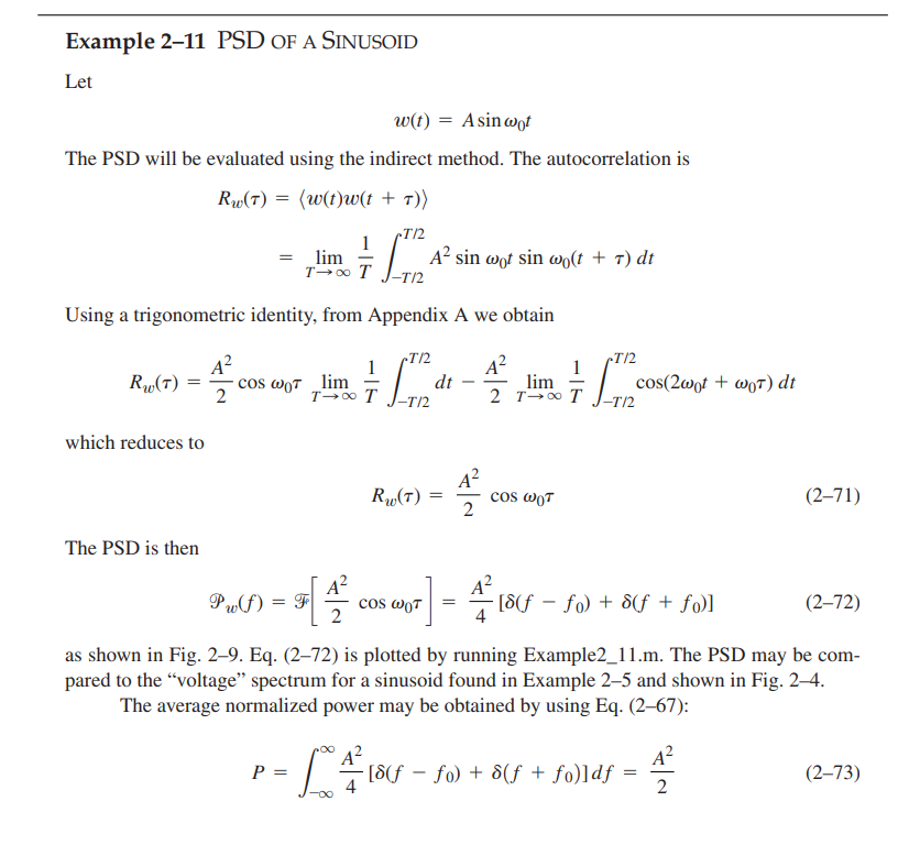
Remember: impulse scaling
\[ \cos(2\pi f_0t) \overset{\mathcal{F}}{\longrightarrow} \frac{1}{2}[\delta(f -f_0)+\delta(f+f_0)] \]
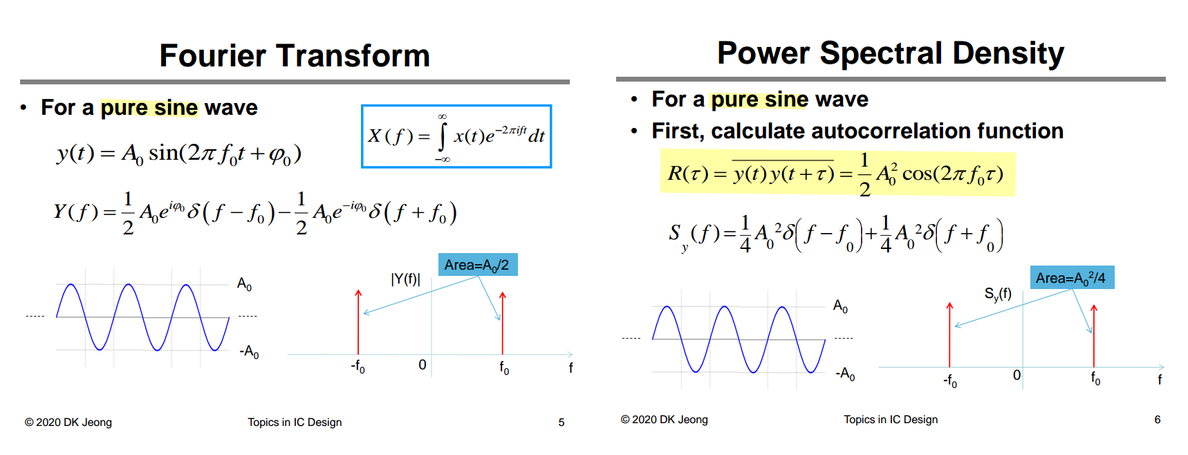
| \(x(t)\) | \(R(\tau)\) |
|---|---|
| \(A_0 \sin(\omega_0 t+\phi_0)\) | \(\frac{A_0^2}{2}\cos(\omega_0 \tau)\) |
| \(A_0 \cos(\omega_0 t+\phi_0)\) | \(\frac{A_0^2}{2}\cos(\omega_0 \tau)\) |
due to \(\cos(\omega_0 t +\phi_0) = \sin(\omega_0 t +\phi_0 + \frac{\pi}{2})\)
Discrete time
Diniz PSR, da Silva EAB, Netto SL. Digital Signal Processing: System Analysis and Design. 2nd ed. Cambridge University Press; 2010.
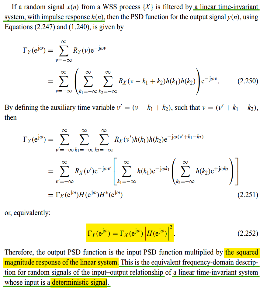
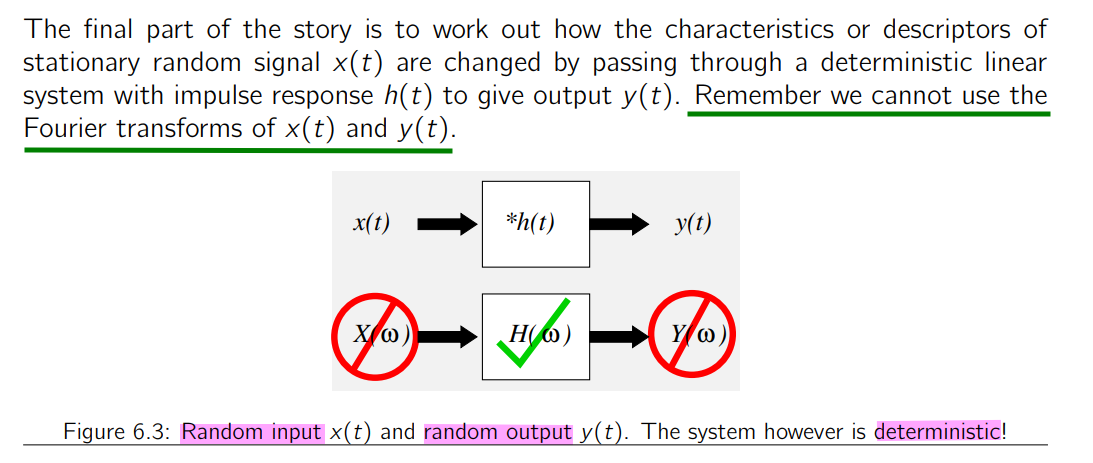
filtered by a linear time-invariant system
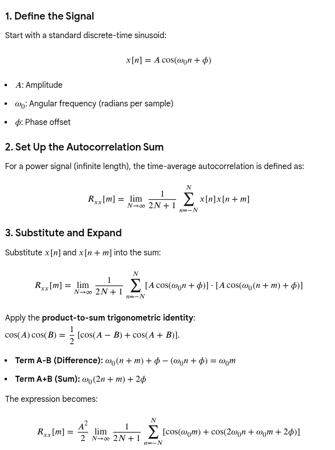
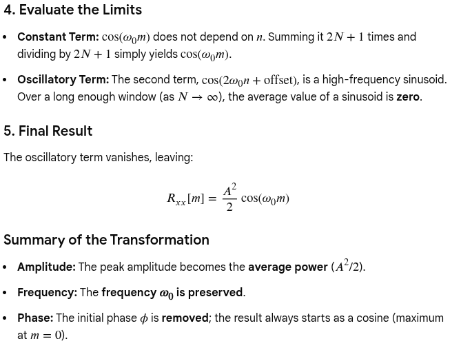
ACF of discrete-time sinusoid. Google AI Mode [https://share.google/aimode/IHyr7o8jLUMx2Leb3]
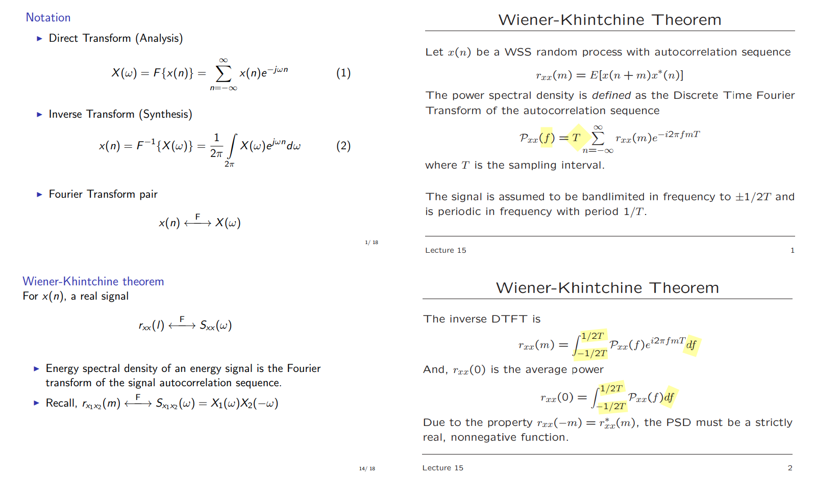
SIMG-713 Noise and Random Processes Spring 2002 . Lecture 15 Power Spectrum Estimation [https://www.cis.rit.edu/class/simg713/Lectures/Lecture713-15-4.pdf]
Properties of the Fourier Transform for Discrete-Time Signals [https://www.comm.utoronto.ca/dkundur/course_info/362/EmanHammadDTFT2.pdf]
 \[
\frac{1}{2\pi}F^{-1}\{R_{xx}\}d\omega =
\frac{1}{2\pi}F^{-1}\{R_{xx}\}d(2\pi f T)=T\cdot F^{-1}\{R_{xx}\}df =
P_{xx}(f)df
\] power spectral density of a discrete-time
random process \(\{x(n)\}\) is
given by \[
P_{xx}(f) =T\cdot F^{-1}\{R_{xx}\}
\]
\[
\frac{1}{2\pi}F^{-1}\{R_{xx}\}d\omega =
\frac{1}{2\pi}F^{-1}\{R_{xx}\}d(2\pi f T)=T\cdot F^{-1}\{R_{xx}\}df =
P_{xx}(f)df
\] power spectral density of a discrete-time
random process \(\{x(n)\}\) is
given by \[
P_{xx}(f) =T\cdot F^{-1}\{R_{xx}\}
\]
PSD & ESD
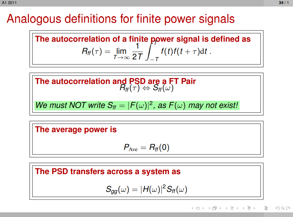
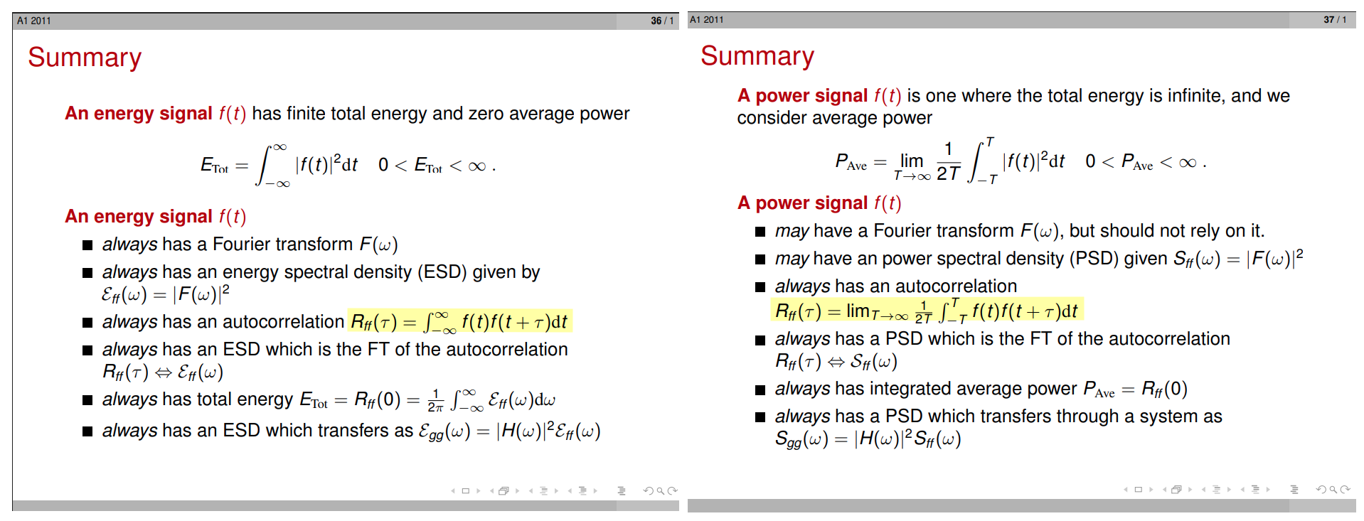
David Murray. Topic 5 Energy & Power Spectra, and Correlation [https://www.robots.ox.ac.uk/~dwm/Courses/2TF_2011/2TF-L5.pdf]
Finite Energy signals & Finite Power signals
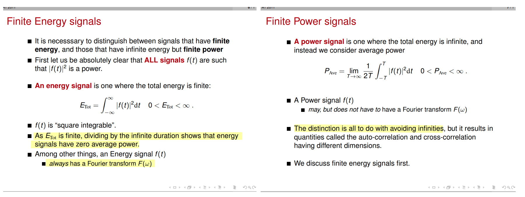
2.161 Signal Processing - Continuous and Discrete Fall Term 2008 Lecture 22 [pdf]
Sklar, Bernard. Digital communications: fundamentals and applications. Pearson, 2021.
LTI Filtering of WSS process
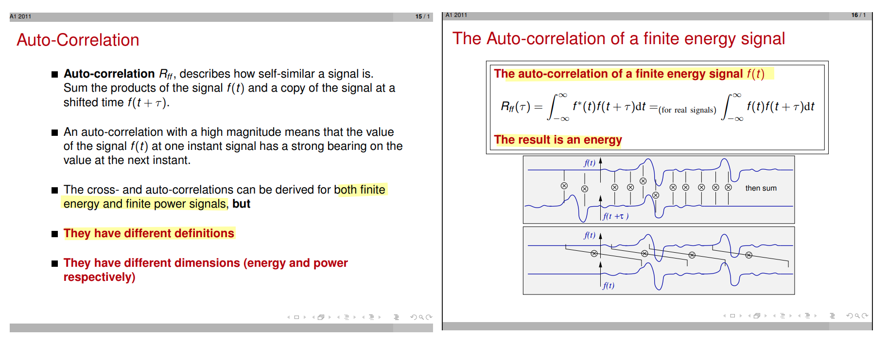
CT Deterministic Autocorrelation Function
Topic 6 Random Processes and Signals [https://www.robots.ox.ac.uk/~dwm/Courses/2TF_2021/N6.pdf]
Alan V. Oppenheim, Introduction To Communication, Control, And Signal Processing [https://ocw.mit.edu/courses/6-011-introduction-to-communication-control-and-signal-processing-spring-2010/a6bddaee5966f6e73450e6fe79ab0566_MIT6_011S10_notes.pdf]
Balu Santhanam, Probability Theory & Stochastic Process 2020: LTI Systems and Random Signals [https://ece-research.unm.edu/bsanthan/ece541/LTI.pdf]
 \[
R_{yy}(\tau) = h(\tau)*R_{xx}(\tau)*h(-\tau)
=R_{xx}(\tau)*h(\tau)*h(-\tau)
\]
\[
R_{yy}(\tau) = h(\tau)*R_{xx}(\tau)*h(-\tau)
=R_{xx}(\tau)*h(\tau)*h(-\tau)
\]
why \(\overline{R}_{hh}(\tau) \overset{\Delta}{=} h(\tau)*h(-\tau)\) is autocorrelation ? the proof is as follows:
\[\begin{align} \overline{R}_{hh}(\tau) &= h(\tau)*h(-\tau) \\ &= \int_{-\infty}^{\infty}h(x)h(-(\tau - x))dx \\ &= \int_{-\infty}^{\infty}h(x)h(-\tau + x)dx \\ &=\int_{-\infty}^{\infty}h(x+\tau)h(x)dx \end{align}\]
Time Reversal \[ x(-t) \overset{FT}{\longrightarrow} X(-j\omega) \]
if \(x(t)\) is real, then \(X(j\omega)\) has conjugate symmetry \[ X(-j\omega) = X^*(j\omega) \]
DT Deterministic Autocorrelation Function
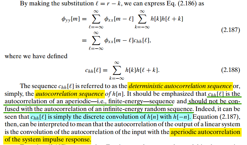
\[
c_{hh}[l] =
\sum_{k=-\infty}^{\infty}h[k]h[l+k]=\sum_{k=-\infty}^{\infty}h[-l+k]h[k]=\sum_{k=-\infty}^{\infty}h[-(l-k)]h[k]=h[l]*h[-l]
\] 
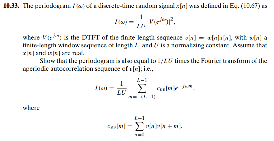
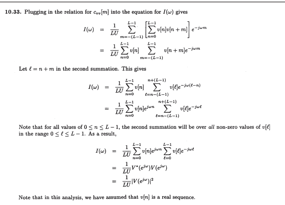
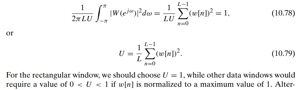
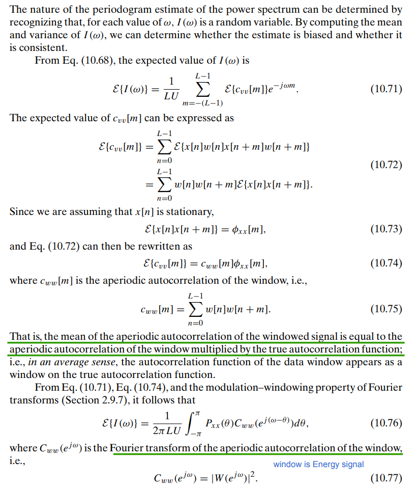
Periodogram
The periodogram is in fact the Fourier transform of the aperiodic correlation of the windowed data sequence
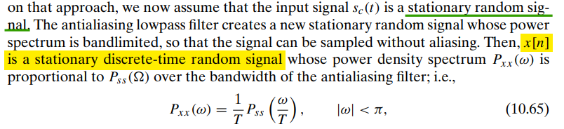
estimating continuous-time stationary random signal

The sequence \(x[n]\) is typically multiplied by a finite-duration window \(w[n]\), since the input to the DFT must be of finite duration. This produces the finite-length sequence \(v[n] = w[n]x[n]\)
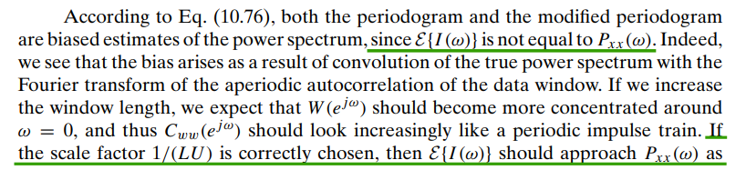
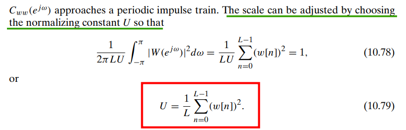
\[\begin{align} \hat{P}_{ss}(\Omega) &= \frac{|V(e^{j\omega})|^2}{LU} \\ &= \frac{|V(e^{j\omega})|^2}{\sum_{n=0}^{L-1}(w[n])^2} \tag{1}\\ &= \frac{L|V(e^{j\omega})|^2}{\sum_{k=0}^{L-1}(W[k])^2} \tag{2} \end{align}\]
That is, by \((1)\) \[ \hat{P}_{ss}(\Omega) = T_s\hat{P}_{xx(\omega)} = \frac{T_s|V(e^{j\omega})|^2}{\sum_{n=0}^{L-1}(w[n])^2}=\frac{|V(e^{j\omega})|^2}{f_{res}L\sum_{n=0}^{L-1}(w[n])^2} \]
That is, by \((2)\) \[ \hat{P}_{ss}(\Omega) = T_s\hat{P}_{xx(\omega)} = \frac{T_sL|V(e^{j\omega})|^2}{\sum_{k=0}^{L-1}(W[k])^2} = \frac{|V(e^{j\omega})|^2}{f_{res}\sum_{k=0}^{L-1}(W[k])^2} \]
!! ENBW
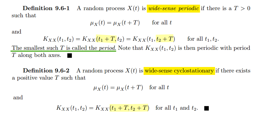
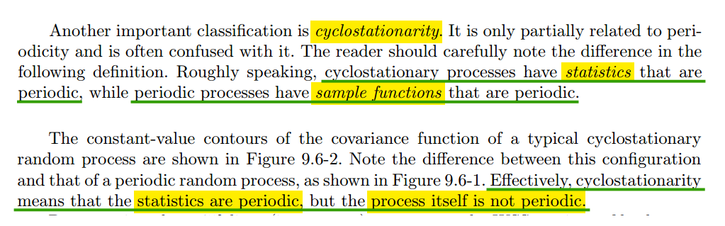
Periodic & Cyclostationary Processes
Multirate Systems & Random Sequences
Balu Santhanam. ece541 Probability Theory & Stochastic Process: Random Signals and Multirate Systems [http://ece-research.unm.edu/bsanthan/ece541/rand.pdf]
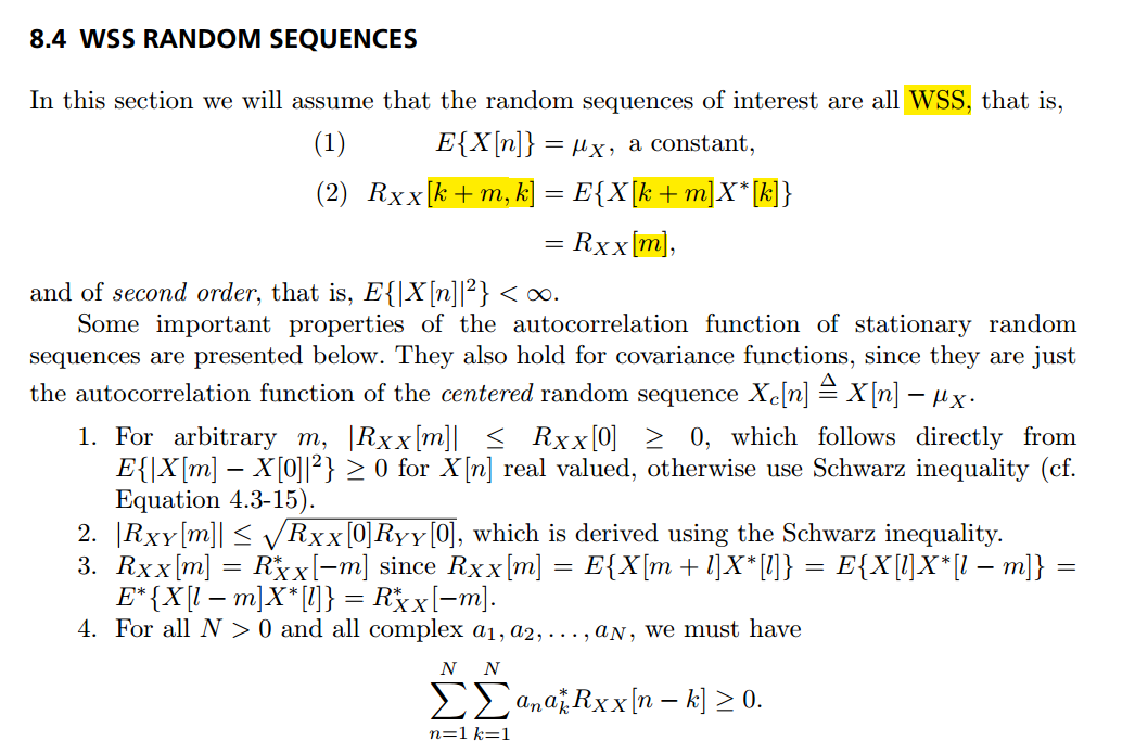
WSS Random Sequences
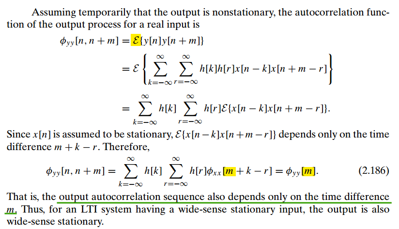
autocorrelation function of WSS random sequences
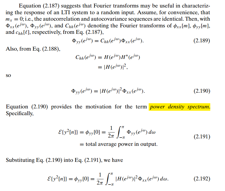
psd of WSS of WSS random sequences
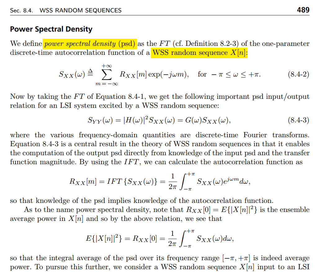
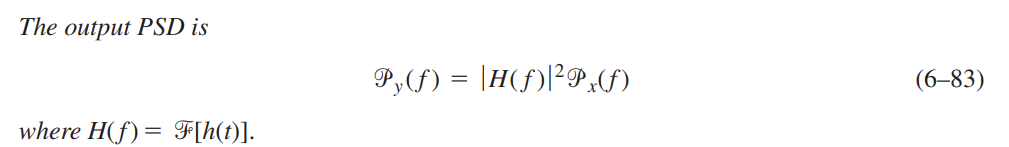
Interpretation of the psd
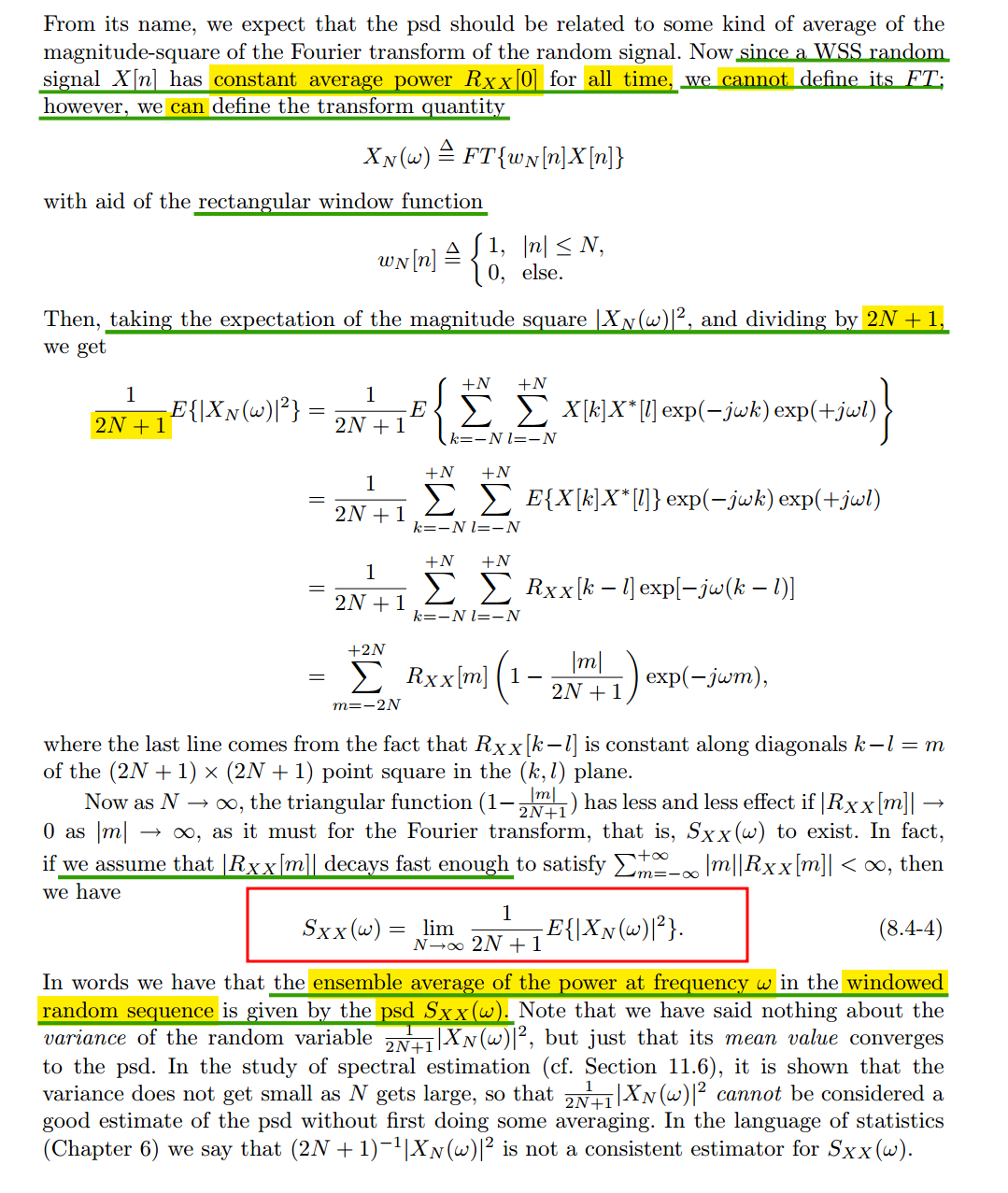
Equation 8.4-4 is permissible for cyclostationary waveforms
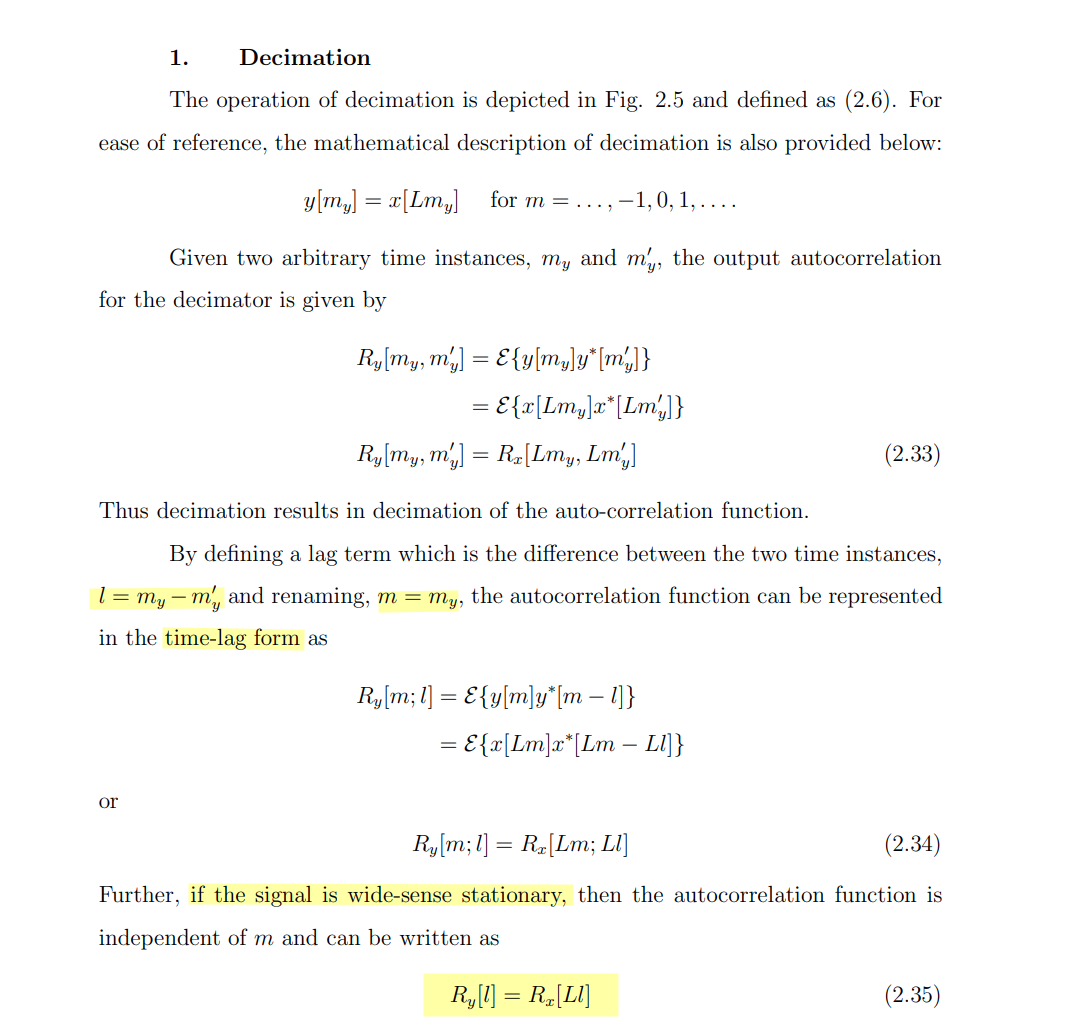
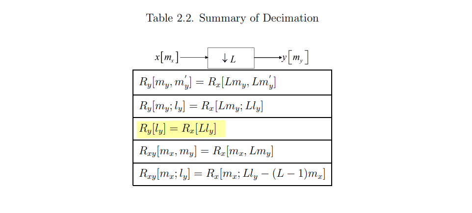
decimation
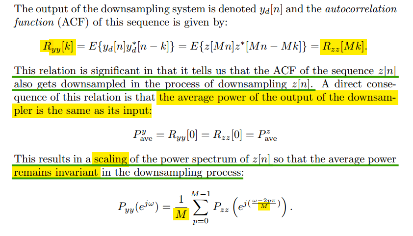
\[ \frac{1}{M}\int_{-Mx_0}^{Mx_0}f(\frac{x}{M})dx = \int_{-Mx_0}^{Mx_0}f(\frac{x}{M}) d\frac{x}{M} = \int_{-x_0}^{x_0} f(\acute{x}) d\acute{x} \]
where \(\acute{x} = \frac{x}{M}\)

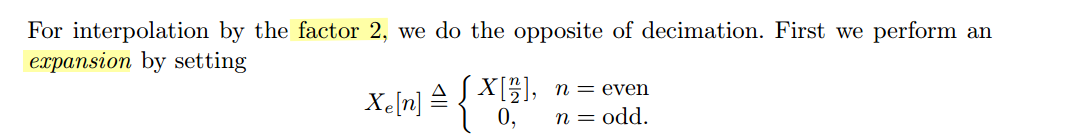
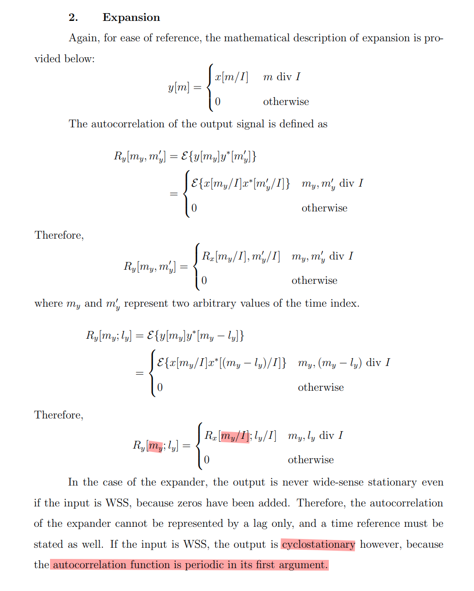
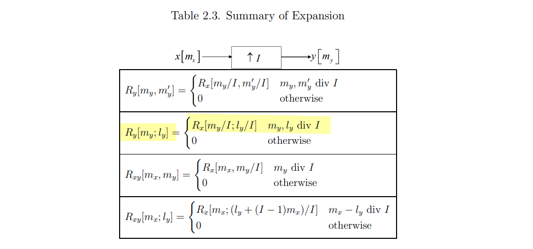
interpolation
The resulting expanded random sequence is clearly nonstationary, because of the zero insertions.
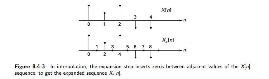
This random sequences and processes is classified as being cyclostationary
psd of \(X_e[n]\), the expansion or the upsampled version of \(X[n]\)
\[ S_{X_eX_e}(\omega) = \frac{1}{L}S_{XX}(L\omega) \]
where \(L\) is upsampling factor
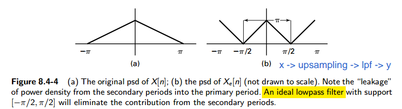
apply \(X_e[n]\) to an ideal lowpass filter with bandwidth \([-\pi/2 , +\pi/2]\) and gain of \(2\) or \(L\)
\[ S_{YY}(\omega) = \left\{ \begin{array}{cl} L \cdot S_{XX}(L\omega), &\ |\omega|\leq \pi/L \\ 0, &\ \pi/L \lt |\omega| \leq \pi \end{array} \right. \]
Stark H, Woods JW. Probability, Statistics, and Random Processes for Engineers, 3rd [pdf]
—, 3th Ed Solution Manual [https://www.scribd.com/document/353335818/Stark-Woods-3th-Ed-Manual#page=212]
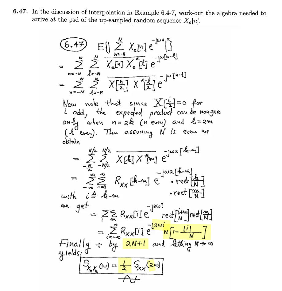
General case with upsampling factor \(L\)
\[\begin{align} &\mathrm{E}\{|\sum_{n=-N}^N X_e[n]e^{-j\omega n}|^2\}\\ &= \sum_{n=-N}^N\sum_{l=-N}^NX_e[n]\cdot X_e^*[l]\cdot e^{-j\omega(n-l)}\\ &= \sum_{n=-N}^N\sum_{l=-N}^NX[\frac{n}{L}]\cdot X^*[\frac{l}{L}]\cdot e^{-j\omega(n-l)}\\ &= \sum_{k=-N/L}^{N/L}\sum_{m=-N/L}^{N/L}X[k]\cdot X^*[m]\cdot e^{-jL\omega (k-m)}\\ &= \sum_{k=-\infty}^{\infty}\sum_{m=-\infty}^{\infty}R_{XX}[k-m]\cdot e^{-j\omega L(k-m)}\cdot \mathcal{rect}[\frac{k}{2N/L}]\cdot \mathcal{rect}[\frac{m}{2N/L}]\\ &= \sum_{i=-\infty}^{\infty}\sum_{m=-\infty}^{\infty}R_{XX}[i]\cdot e^{-jL\omega i}\cdot \mathcal{rect}[\frac{i+m}{2N/L}]\cdot \mathcal{rect}[\frac{m}{2N/L}]\\ &= \sum_{i=-\infty}^{\infty}R_{XX}[i]\cdot e^{-jL\omega i} \cdot \frac{2N}{L}\left[1 -\frac{|i|}{2N/L} \right] \end{align}\]
Then \[\begin{align} S_{X_eX_e}(\omega) &= \lim_{N\to \infty}\frac{1}{2N+1}\cdot \mathrm{E}\{|\sum_{n=-N}^N X_e[n]e^{-j\omega n}|^2\} \\ &= \frac{1}{L}\sum_{i=-\infty}^{\infty}R_{XX}[i]\cdot e^{-jL\omega i}\\ &= \frac{1}{L}S_{XX}(L\omega) \end{align}\]
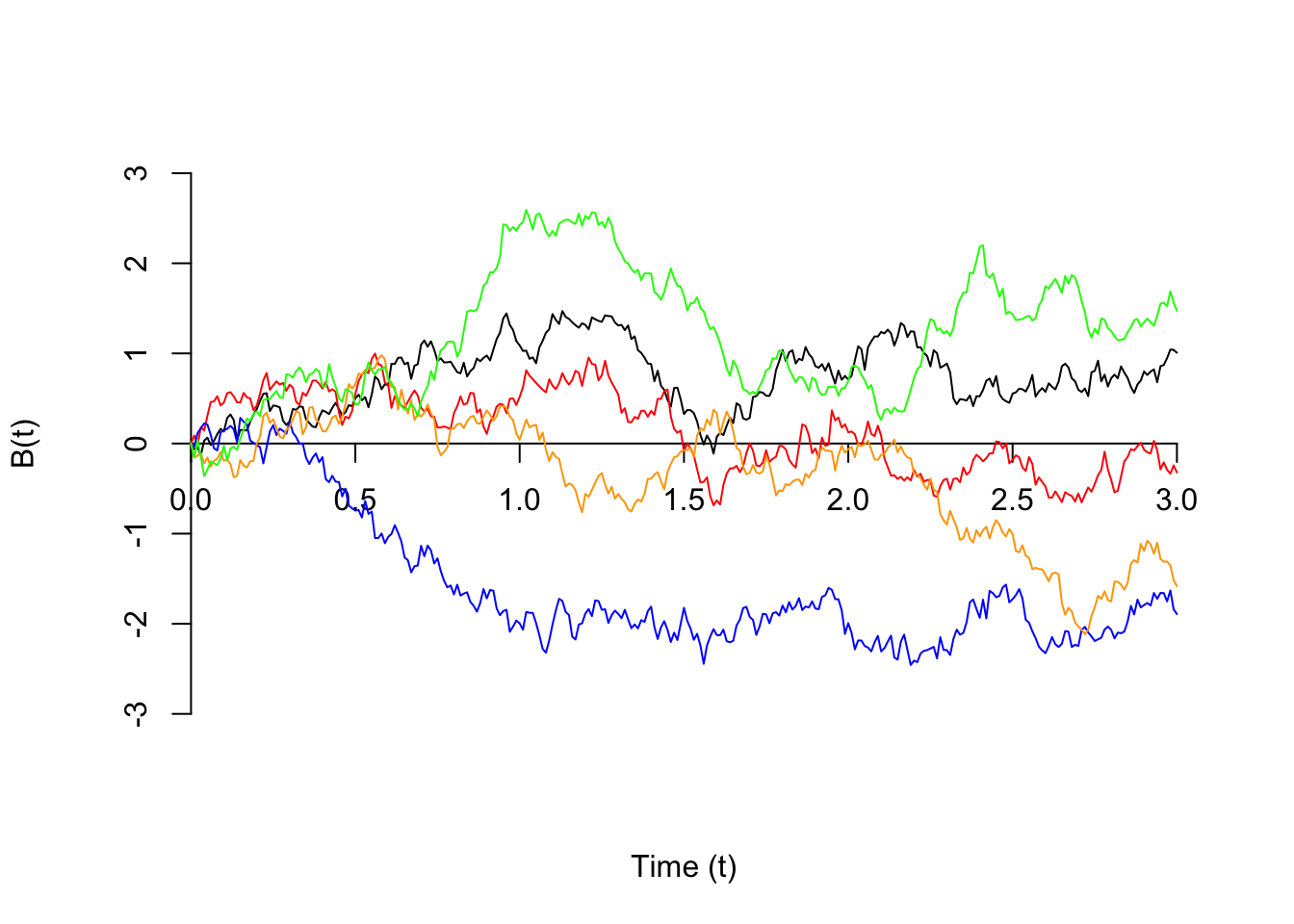
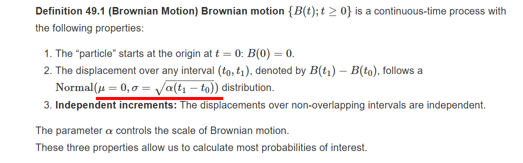
Wiener Process (Brownian Motion)
Dennis Sun, Introduction to Probability: Lesson 49 Brownian Motion [https://dlsun.github.io/probability/brownian-motion.html]
Wiener process (also called Brownian motion)
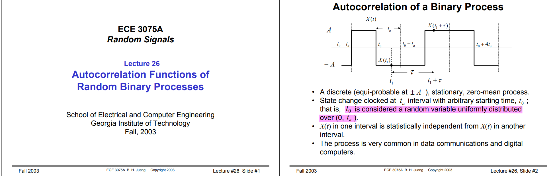
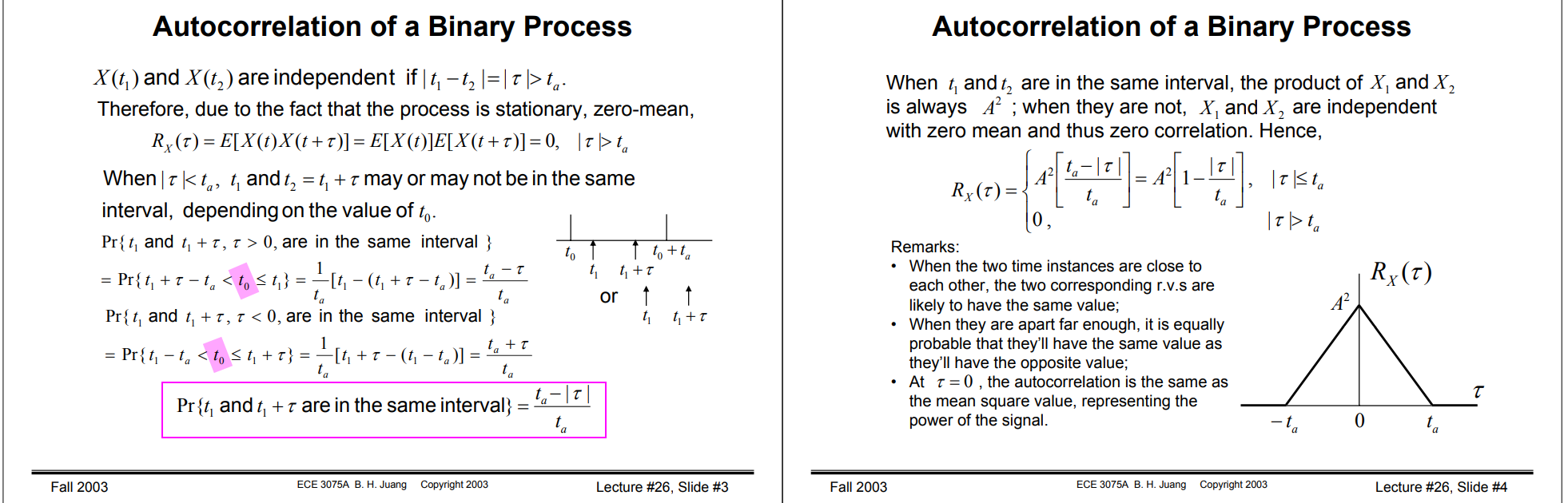
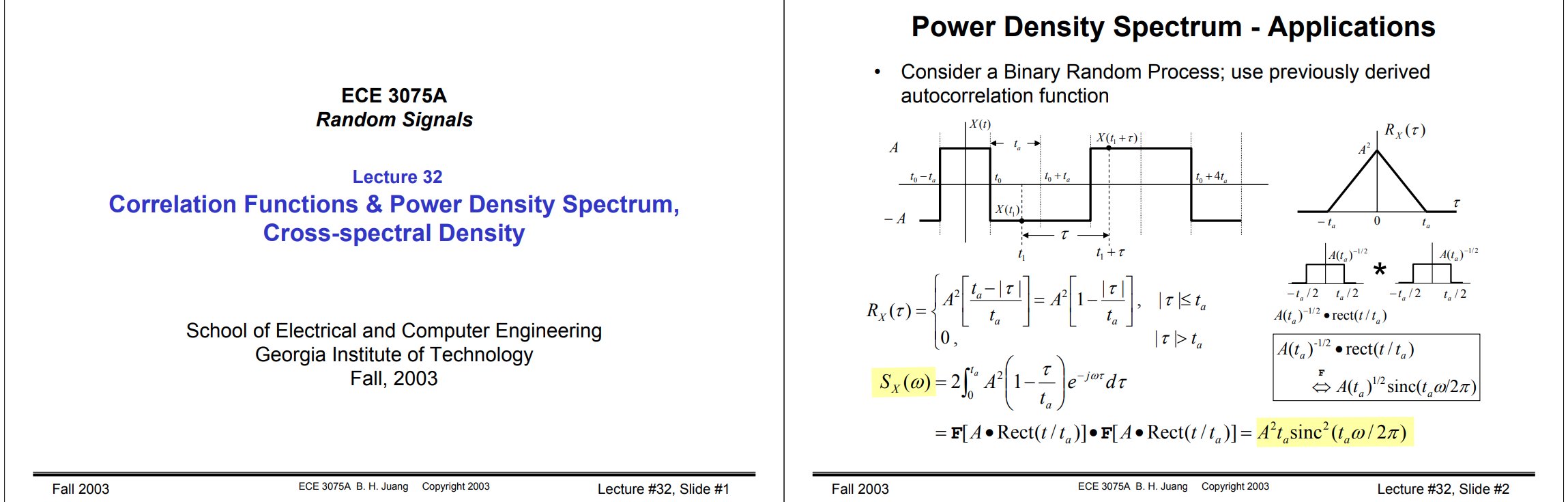
NRZ PSD
Lecture 26 Autocorrelation Functions of Random Binary Processes [https://bpb-us-e1.wpmucdn.com/sites.gatech.edu/dist/a/578/files/2003/12/ECE3075A-26.pdf]
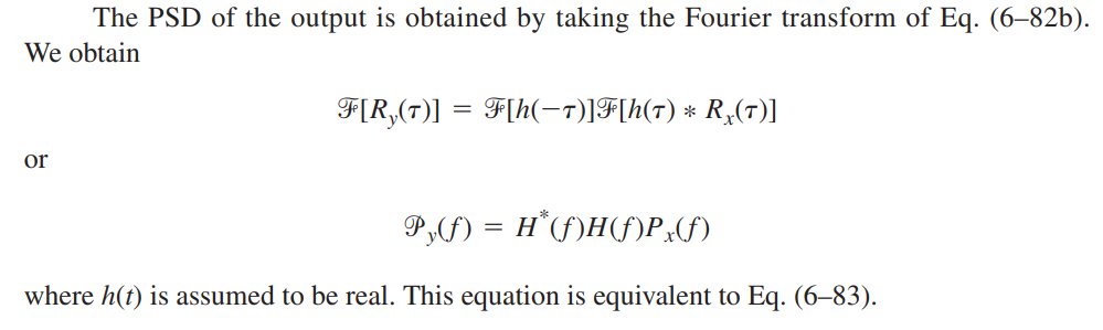
Lecture 32 Correlation Functions & Power Density Spectrum, Cross-spectral Density [https://bpb-us-e1.wpmucdn.com/sites.gatech.edu/dist/a/578/files/2003/12/ECE3075A-32.pdf]
note \(\color{red}S_x(0)=0\)
Normal Distribution and Input-Referred Noise [https://a2d2ic.wordpress.com/2013/06/05/normal-distribution-and-input-referred-noise/]
![Fig.2 The noise signal, its auto correlation function, and spectral density [2]](/2023/11/10/random/trnoise.jpg)
reference
L.W. Couch, Digital and Analog Communication Systems, 8th Edition, 2013 [pdf]
Alan V Oppenheim, George C. Verghese, Signals, Systems and Inference, 1st edition [pdf]
R. Ziemer and W. Tranter, Principles of Communications, Seventh Edition, 2013 [pdf]
Stark H, Woods JW. Probability, Statistics, and Random Processes for Engineers, 4th ed. 2012 [pdf]
Kuchler, Ryan J. Theory of multirate statistical signal processing and applications. Monterey, California.: Naval Postgraduate School, 2005. [pdf]
Balu Santhanam. Fall 2020 ECE541 Probability Theory & Stochastic Process [https://ece-research.unm.edu/bsanthan/ece541/]