Linear Circuits Analysis
Are AC-Driven Circuits Linear?
\[ f(x_1 + x_2)= f(x_1)+ f(x_2) \]
Often, AC-driven circuits can be mistaken as non-linear as the basis that determines the linearity of a circuit is the relationship between the voltage and current.
While an AC signal varies with time, it still exhibits a linear relationship across elements like resistors, capacitors, and inductors. Therefore, AC driven circuits are linear.
Phasor
Phasor concept has no real physical significance. It is just a convenient mathematical tool.
Phasor analysis determines the steady-state response to a linear circuit driven by sinusoidal sources with frequency \(f\)
If your circuit includes transistors or other nonlinear components, all is not lost. There is an extension of phasor analysis to nonlinear circuits called small-signal analysis in which you linearize the components before performing phasor analysis - AC analyses of SPICE
A sinusoid is characterized by 3 numbers, its amplitude, its phase, and its frequency. For example \[ v(t) = A\cos(\omega t + \phi) \tag{1} \] In a circuit there will be many signals but in the case of phasor analysis they will all have the same frequency. For this reason, the signals are characterized using only their amplitude and phase.
The combination of an amplitude and phase to describe a signal is the phasor for that signal.
Thus, the phasor for the signal in \((1)\) is \(A\angle \phi\)
In general, phasors are functions of frequency
Often it is preferable to represent a phasor using complex numbers rather than using amplitude and phase. In this case we represent the signal as: \[ v(t) = \Re\{Ve^{j\omega t} \} \tag{2} \] where \(V=Ae^{j\phi}\) is the phasor.
\((1)\) and \((2)\) are the same
Phasor Model of a Resistor
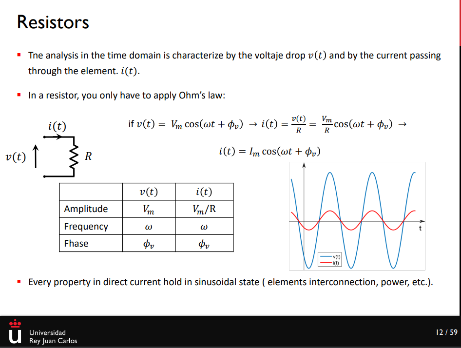
A linear resistor is defined by the equation \(v = Ri\)
Now, assume that the resistor current is described with the phasor \(I\). Then \[ i(t) = \Re\{Ie^{j\omega t}\} \] \(R\) is a real constant, and so the voltage can be computed to be \[ v(t) = R\Re\{Ie^{j\omega t}\} = \Re\{RIe^{j\omega t}\} = \Re\{Ve^{j\omega t}\} \] where \(V\) is the phasor representation for \(v\), i.e. \[ V = RI \]
Thus, given the phasor for the current we can directly compute the phasor for the voltage across the resistor.
Similarly, given the phasor for the voltage across a resistor we can compute the phasor for the current through the resistor using \(I = \frac{V}{R}\)
Phasor Model of a Capacitor
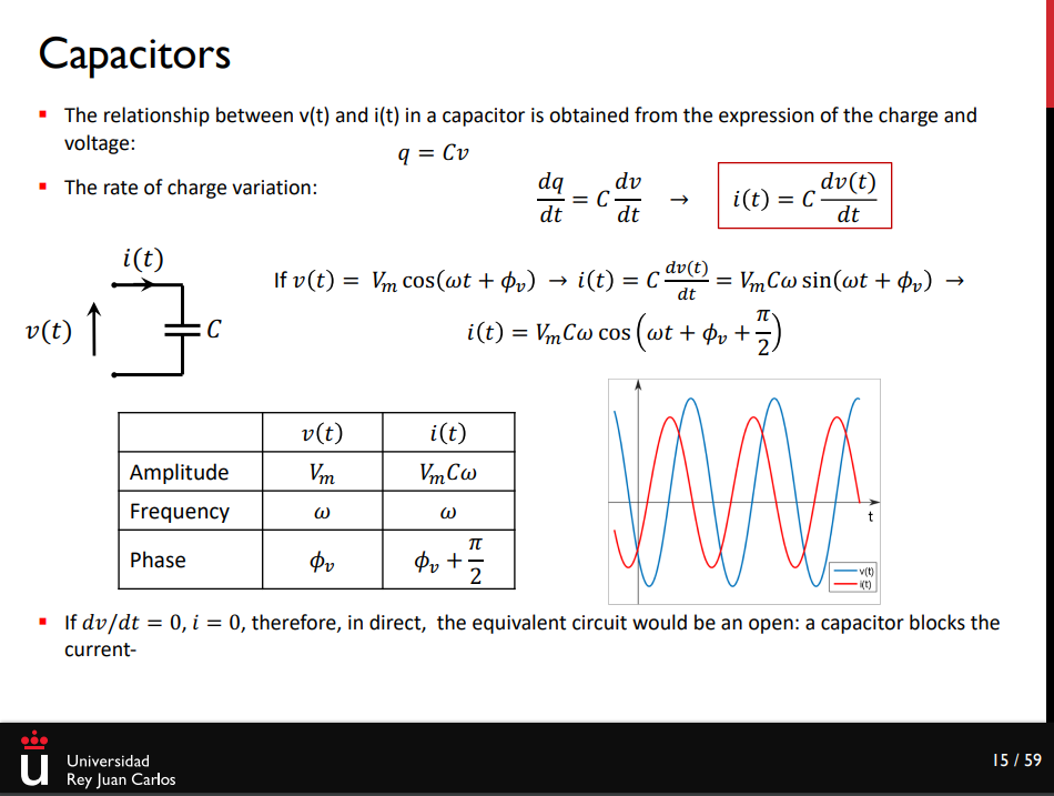
A linear capacitor is defined by the equation \(i=C\frac{dv}{dt}\)
Now, assume that the voltage across the capacitor is described with the phasor \(V\). Then \[ v(t) = \Re\{ V e^{j\omega t}\} \] \(C\) is a real constant \[ i(t) = C\Re\{\frac{d}{dt}V e^{j\omega t}\} = \Re\{j\omega C V e^{j\omega t}\} \] The phasor representation for \(i\) is \(i(t) = \Re\{Ie^{j\omega t}\}\), that is \(I = j\omega C V\)
Thus, given the phasor for the voltage across a capacitor we can directly compute the phasor for the current through the capacitor.
Similarly, given the phasor for the current through a capacitor we can compute the phasor for the voltage across the capacitor using \(V=\frac{I}{j\omega C}\)
Phasor Model of an Inductor
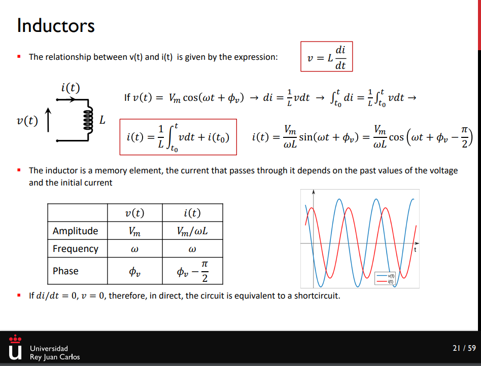
A linear inductor is defined by the equation \(v=L\frac{di}{dt}\)
Now, assume that the inductor current is described with the phasor \(I\). Then \[ i(t) = \Re\{ I e^{j\omega t}\} \] \(L\) is a real constant, and so the voltage can be computed to be \[ v(t) = L\Re\{\frac{d}{dt}I e^{j\omega t}\} = \Re\{j\omega L I e^{j\omega t}\} \] The phasor representation for \(v\) is \(v(t) = \Re\{Ve^{j\omega t}\}\), that is \(V = j\omega L I\)
Thus, given the phasor for the current we can directly compute the phasor for the voltage across the inductor.
Similarly, given the phasor for the voltage across an inductor we can compute the phasor for the current through the inductor using \(I=\frac{V}{j\omega L}\)
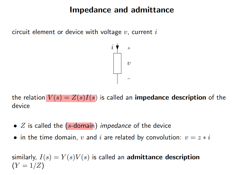
Impedance and Admittance
Impedance and admittance are generalizations of resistance and conductance.
They differ from resistance and conductance in that they are complex and they vary with frequency.
Impedance is defined to be the ratio of the phasor for the voltage across the component and the current through the component: \[ Z = \frac{V}{I} \]
Impedance is a complex value. The real part of the impedance is referred to as the resistance and the imaginary part is referred to as the reactance
For a linear component, admittance is defined to be the ratio of the phasor for the current through the component and the voltage across the component: \[ Y = \frac{I}{V} \]
Admittance is a complex value. The real part of the admittance is referred to as the conductance and the imaginary part is referred to as the susceptance.
Response to Complex Exponentials
The response of an LTI system to a complex exponential input is the same complex exponential with only a change in amplitude
\[\begin{align} y(t) &= H(s)e^{st} \\ H(s) &= \int_{-\infty}^{+\infty}h(\tau)e^{-s\tau}d\tau \end{align}\]
where \(h(t)\) is the impulse response of a continuous-time LTI system
convolution integral is used here
\[\begin{align} y[n] &= H(z)z^n \\ H(z) &= \sum_{k=-\infty}^{+\infty}h[k]z^{-k} \end{align}\]
where \(h(n)\) is the impulse response of a discrete-time LTI system
convolution sum is used here
The signals of the form \(e^{st}\) in continuous time and \(z^{n}\) in discrete time, where \(s\) and \(z\) are complex numbers are referred to as an eigenfunction of the system, and the amplitude factor \(H(s)\), \(H(z)\) is referred to as the system's eigenvalue
Laplace transform
One of the important applications of the Laplace transform is in the analysis and characterization of LTI systems, which stems directly from the convolution property \[ Y(s) = H(s)X(s) \] where \(X(s)\), \(Y(s)\), and \(H(s)\) are the Laplace transforms of the input, output, and impulse response of the system, respectively
From the response of LTI systems to complex exponentials, if the input to an LTI system is \(x(t) = e^{st}\), with \(s\) the ROC of \(H(s)\), then the output will be \(y(t)=H(s)e^{st}\); i.e., \(e^{st}\) is an eigenfunction of the system with eigenvalue equal to the Laplace transform of the impulse response.
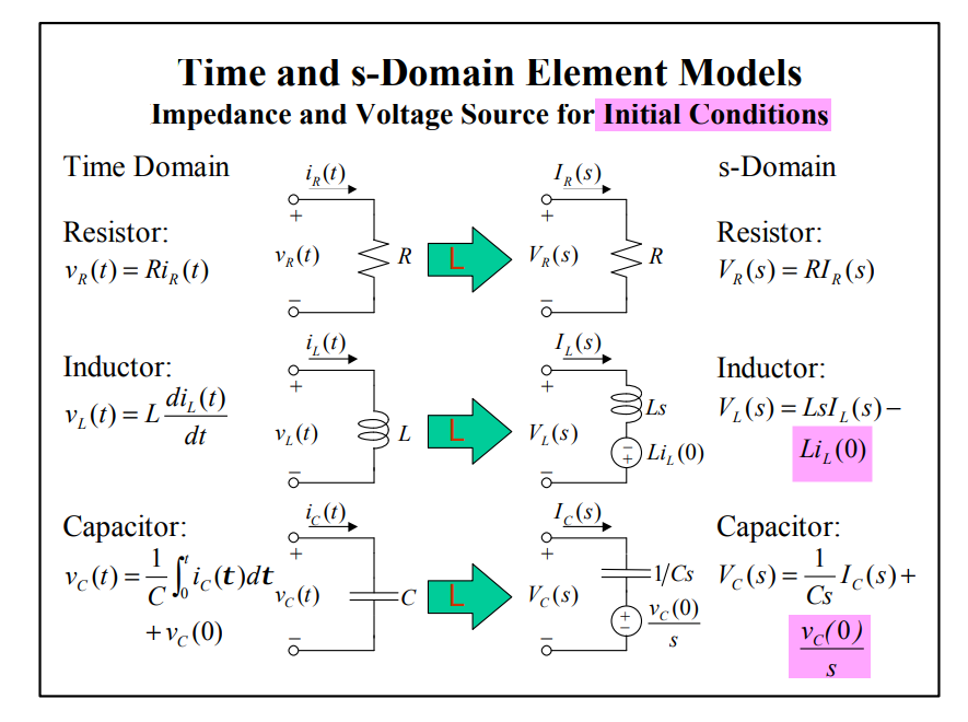
s-Domain Element Models
Sinusoidal Steady-State Analysis
Here Sinusoidal means that source excitations have the form \(V_s\cos(\omega t +\theta)\) or \(V_s\sin(\omega t+\theta)\)
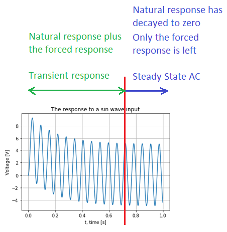
Steady state mean that all transient behavior of the stable circuit has died out, i.e., decayed to zero
\(s\)-domain and phasor-domain
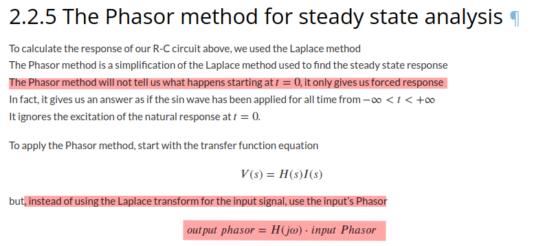
Phasor analysis is a technique to find the steady-state response when the system input is a sinusoid. That is, phasor analysis is sinusoidal analysis.
- Phasor analysis is a powerful technique with which to find the steady-state portion of the complete response.
- Phasor analysis does not find the transient response.
- Phasor analysis does not find the complete response.
The beauty of the phasor-domain circuit is that it is described by algebraic KVL and KCL equations with time-invariant sources, not differential equations of time
The difference here is that Laplace analysis can also give us the transient response
General Response Classifications
zero-input response, zero-state response & complete response
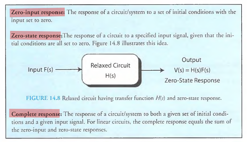
The zero-state response is given by \(\mathscr{L^1}[H(s)F(s)]\), for the arbitrary \(s\)-domain input \(F(s)\)
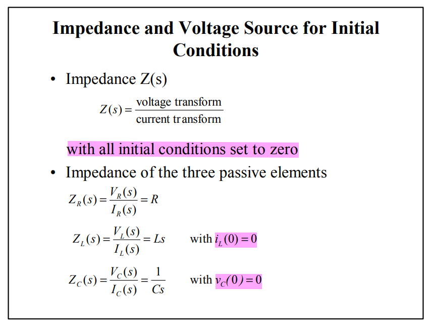
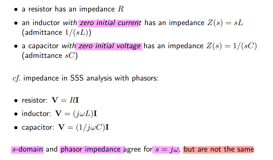
where \(Z_L(s) = sL\), the inductor with zero initial current \(i_L(0)=0\) and \(Z_C(s)=1/sC\) with zero initial voltage \(v_C(0)=0\)
transient response & steady-state response

natural response & forced response

Transfer Functions and Frequency Response
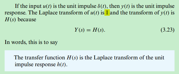
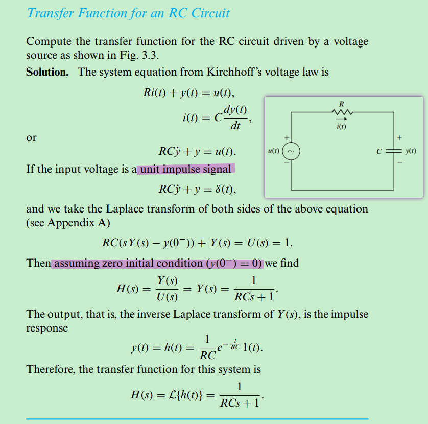
transfer function
The transfer function \(H(s)\) is the ratio of the Laplace transform of the output of the system to its input assuming all zero initial conditions.
frequency response
An immediate consequence of convolution is that an input of the form \(e^{st}\) results in an output \[ y(t) = H(s)e^{st} \] where the specific constant \(s\) may be complex, expressed as \(s = \sigma + j\omega\)
A very common way to use the exponential response of LTIs is in finding the frequency response i.e. response to a sinusoid
First, we express the sinusoid as a sum of two exponential expressions (Euler’s relation): \[ \cos(\omega t) = \frac{1}{2}(e^{j\omega t}+e^{-j\omega t}) \] If we let \(s=j\omega\), then \(H(-j\omega)=H^*(j\omega)\), in polar form \(H(j\omega)=Me^{j\phi}\) and \(H(-j\omega)=Me^{-j\phi}\). \[\begin{align} y_+(t) & = H(s)e^{st}|_{s=j\omega} = H(j\omega)e^{j\omega t} = M e^{j(\omega t + \phi)} \\ y_-(t) & = H(s)e^{st}|_{s=-j\omega} = H(-j\omega)e^{-j\omega t} = M e^{-j(\omega t + \phi)} \end{align}\]
By superposition, the response to the sum of these two exponentials, which make up the cosine signal, is the sum of the responses \[\begin{align} y(t) &= \frac{1}{2}[H(j\omega)e^{j\omega t} + H(-j\omega)e^{-j\omega t}] \\ &= \frac{M}{2}[e^{j(\omega t + \phi)} + e^{-j(\omega t + \phi)}] \\ &= M\cos(\omega t + \phi) \end{align}\]
where \(M = |H(j\omega|\) and \(\phi = \angle H(j\omega)\)
This means if a system represented by the transfer function \(H(s)\) has a sinusoidal input, the output will be sinusoidal at the same frequency with magnitude \(M\) and will be shifted in phase by the angle \(\phi\)
Laplace transform vs. Fourier transform
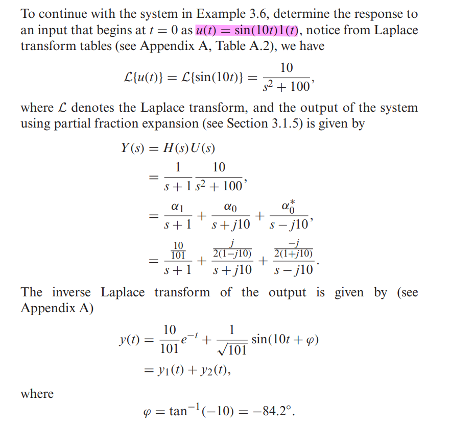
- Laplace transforms such as \(Y(s)=H(s)U(s)\) can be used to study the complete response characteristics of systems, including the transient response—that is, the time response to an initial condition or suddenly applied signal
- This is in contrast to the use of Fourier transforms, which only take into account the steady-state response
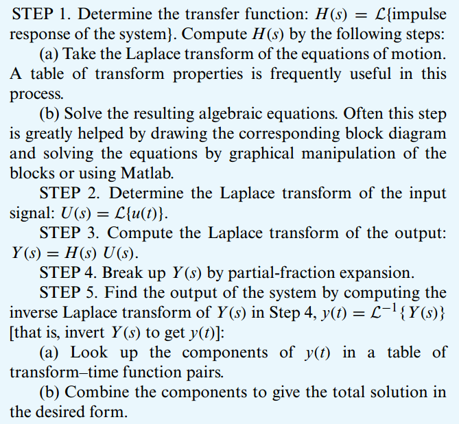
Given a general linear system with transfer function \(H(s)\) and an input signal \(u(t)\), the procedure for determining \(y(t)\) using the Laplace transform is given by the following steps:
Laplace derivative formula at \(t = 0\)
S. Boyd EE102 Table of Laplace Transforms. [https://web.stanford.edu/~boyd/ee102/laplace-table.pdf]
One-Sided (unilateral) and Two-Sided (bilateral) Laplace Transforms
[https://sps.ewi.tudelft.nl/Education/courses/ee2s11/slides/3_laplace_P.pdf]
reference
Ken Kundert. Introduction to Phasors. Designer’s Guide Community. September 2011.
How to Perform Linearity Circuit Analysis [https://resources.pcb.cadence.com/blog/2021-how-to-perform-linearity-circuit-analysis]
Stephen P. Boyd. EE102 Lecture 7 Circuit analysis via Laplace transform [https://web.stanford.edu/~boyd/ee102/laplace_ckts.pdf]
Cheng-Kok Koh, EE695K VLSI Interconnect, S-Domain Analysis [https://engineering.purdue.edu/~chengkok/ee695K/lec3c.pdf]
Kenneth R. Demarest, Circuit Analysis using Phasors, Laplace Transforms, and Network Functions [https://people.eecs.ku.edu/~demarest/212/Phasor%20and%20Laplace%20review.pdf]
DeCarlo, R. A., & Lin, P.-M. (2009). Linear circuit analysis : time domain, phasor, and Laplace transform approaches (3rd ed).
Davis, Artice M.. "Linear Circuit Analysis." The Electrical Engineering Handbook - Six Volume Set (1998)
Duane Marcy, Fundamentals of Linear Systems [http://lcs-vc-marcy.syr.edu:8080/Chapter22.html]
Gene F. Franklin, J. David Powell, and Abbas Emami-Naeini. 2018. Feedback Control of Dynamic Systems (8th Edition) (8th. ed.). Pearson.