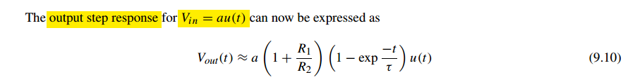
Second-Order System
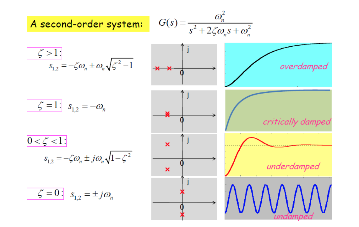
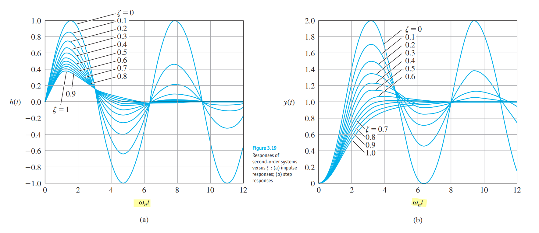
show qualitatively how changing pole locations in the s-plane affect impulse responses

natural frequency (\(\omega_n\), \(\omega_d\))
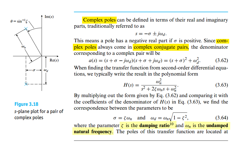
\(\omega_d\) called damped natural frequency \[ \omega_n^2 = \sigma^2 + \omega_d^2 \]
Underdamped step response (\(0<\zeta < 1\))
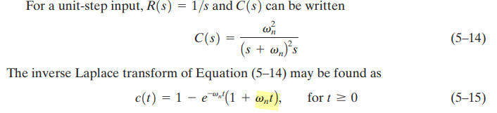
Critically damped step response (\(\zeta =1\))
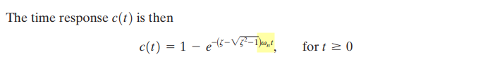
Overdamped step response (\(\zeta >1\))
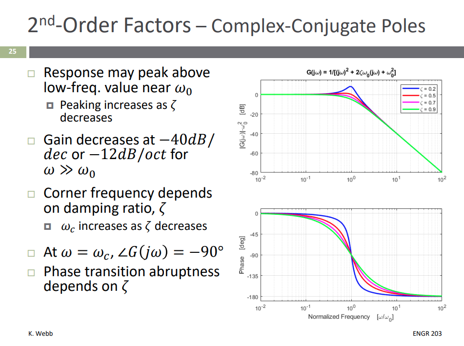
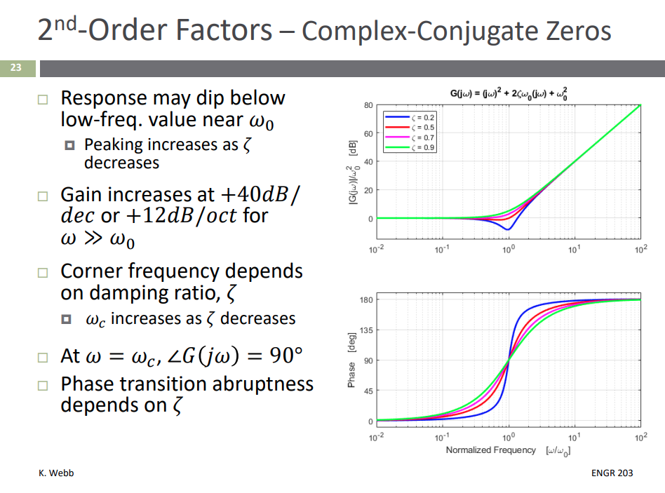
Complex-Conjugate Poles/Zeros
Section 6 Frequency Response Analysis [https://web.engr.oregonstate.edu/~webbky/ENGR203_files/Section%206%20Frequency%20Response%20Analysis.pdf]
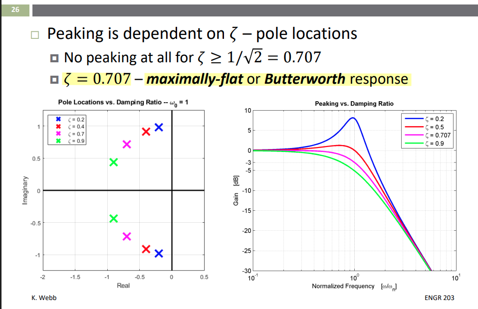
maximally-flat or Butterworth response
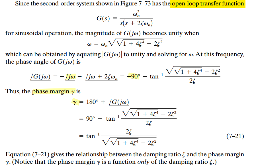
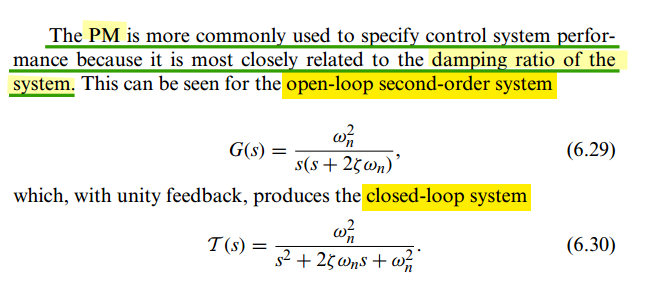
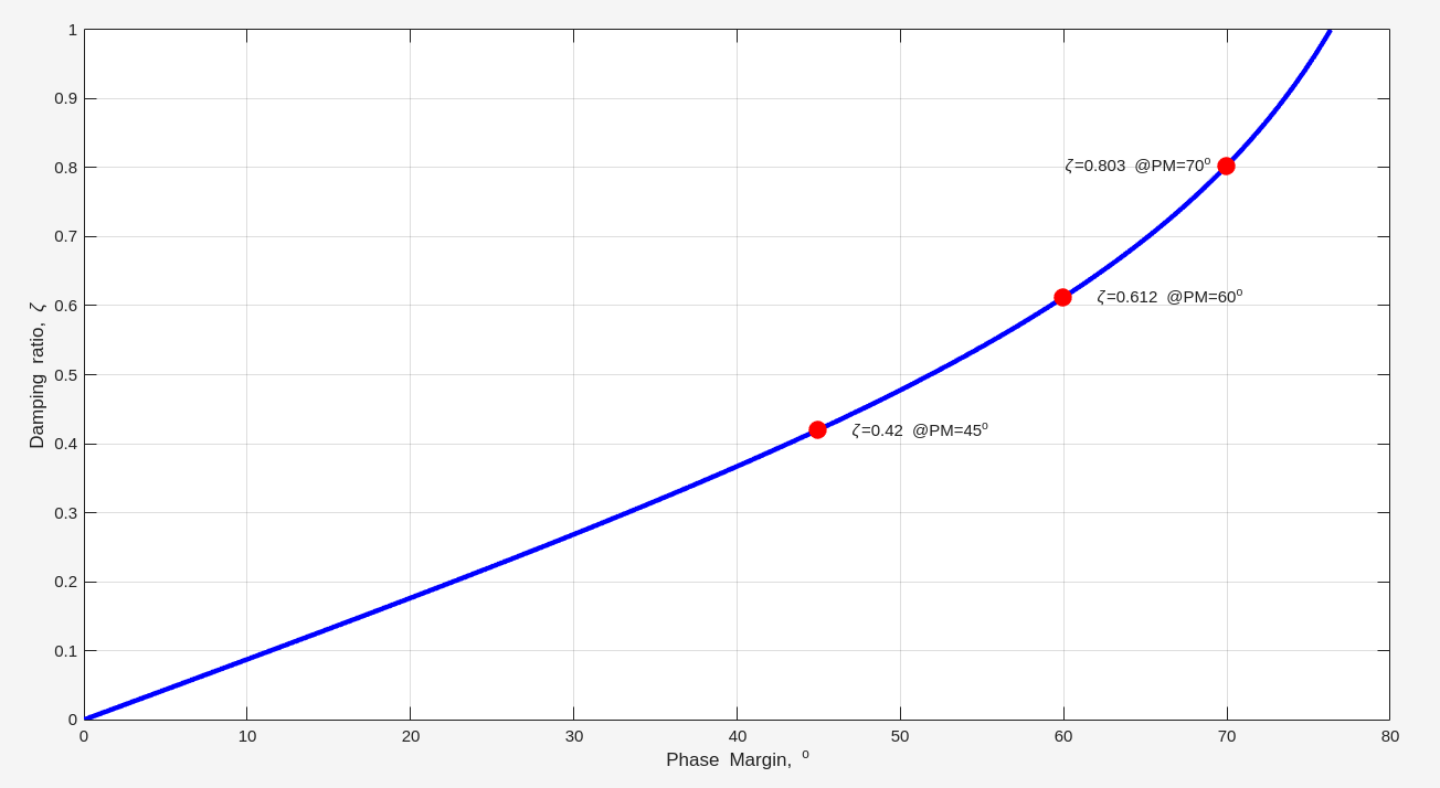
Phase Margin & Damping Factor
Phase Margin is defined for open loop system
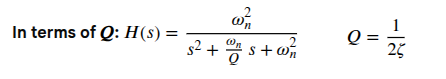
Damping Factor (\(\zeta\)) is defined for close loop system
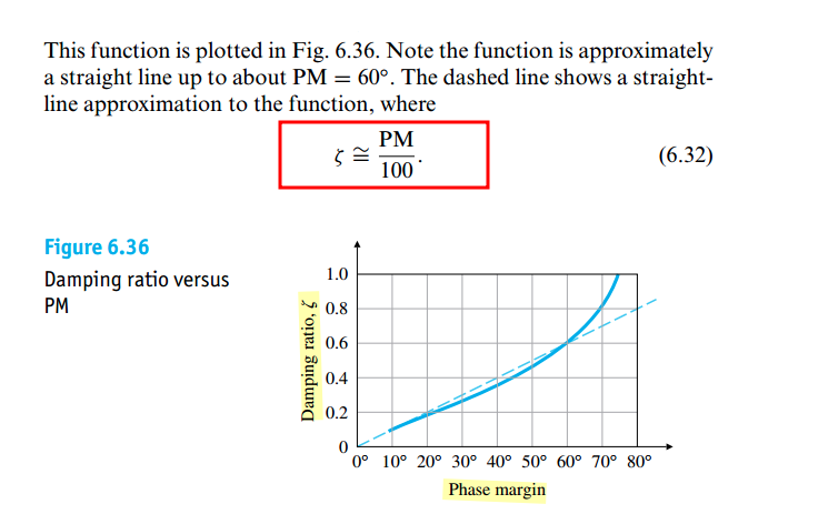
We can analyze open loop system in a better perspective because it is simpler. So, we always use the loop gain analysis to find the phase margin and see whether the system is stable or not.
1 | zta = 0:.001:1; |
Zeros & Non-Minimum Phase Zeros
Influence of Zeros and Non-Minimum Phase Zeros of Transfer Functions on Dynamical System Behavior [https://aleksandarhaber.com/effect-of-zeros-of-transfer-functions-on-dynamical-system-behavior/]
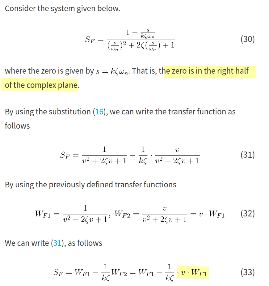
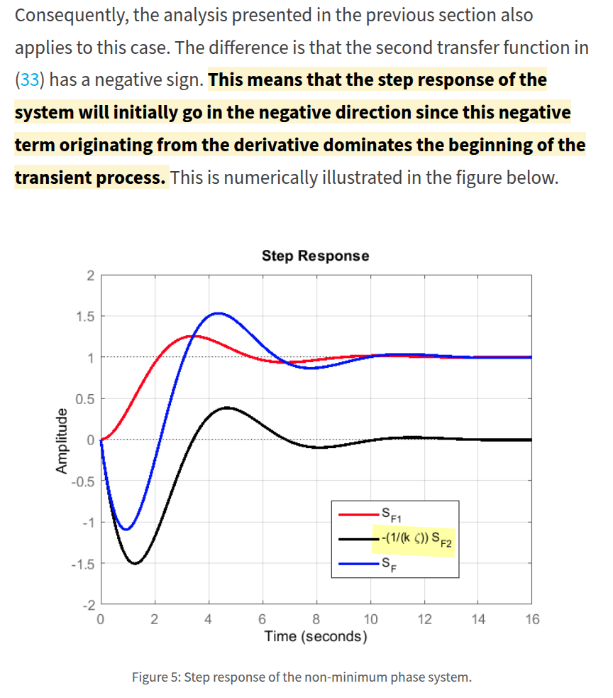
The zeros in the right half of the complex plane are called nonminimum phase zeros. Systems with nonminimum phase zeros are called nonminimum phase systems
Zero close to the real pole attenuates the effect of that pole on the system response
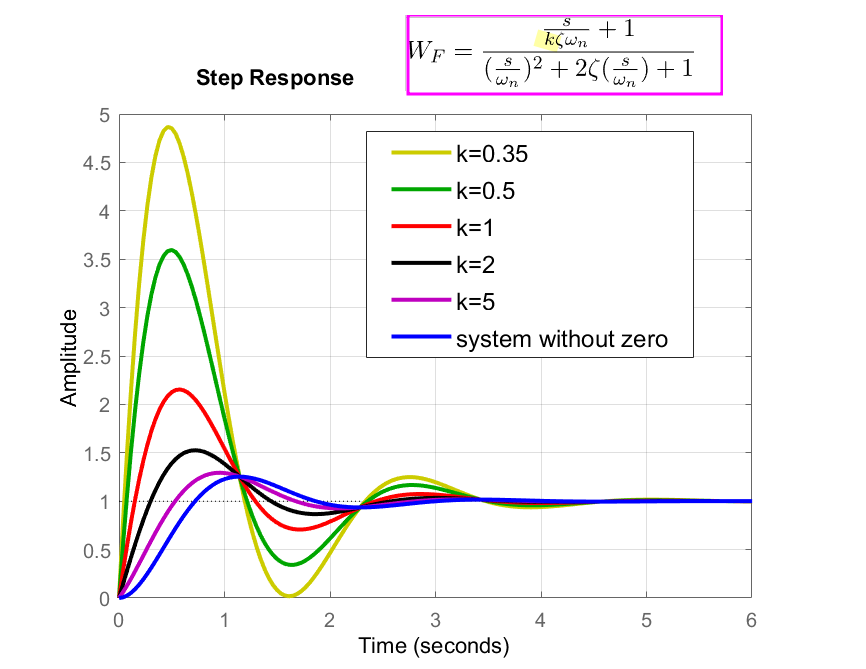
Zeros Tend to Increase the Overshoot of the System
1 | zeta=0.4 |
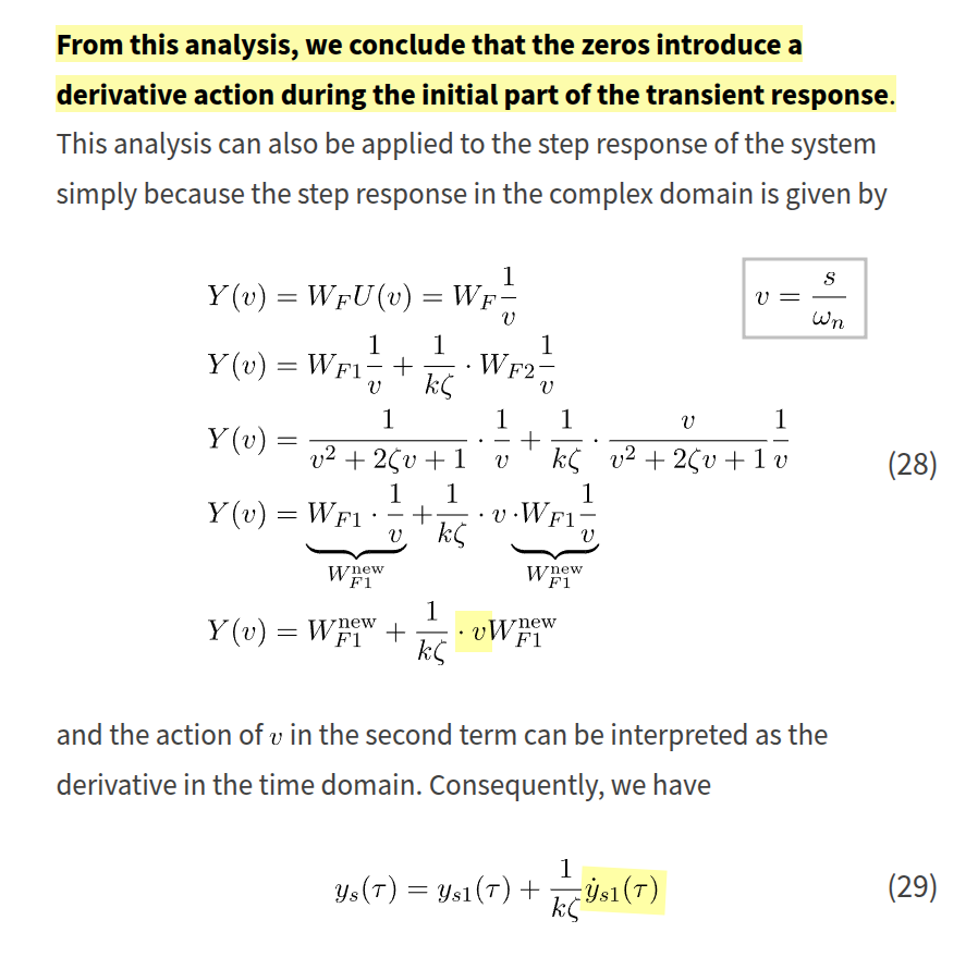
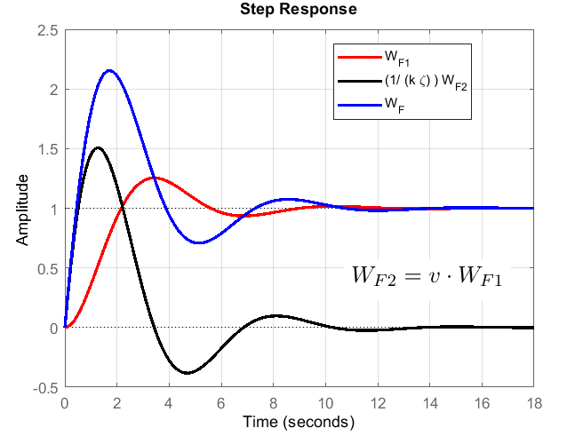
Nonminimum Phase Zeros – Effect on the Transient Response
1 | zeta=0.4 |
\[\begin{align} TF &= \frac{s +\omega_z}{s^2+2\zeta \omega_ns+\omega_n^2} \\ &= \frac{\omega _z}{\omega _n^2}\cdot \frac{1+s/\omega _z}{1+s^2/\omega_n^2+2\zeta s/\omega_n} \end{align}\]
Let \(s=j\omega\) and omit factor, \[ A_\text{dB}(\omega) = 10\log[1+(\frac{\omega}{\omega _z})^2] - 10\log[1+\frac{\omega^4}{\omega_n^4}+\frac{2\omega^2(2\zeta ^2 -1)}{\omega_n^2}] \] peaking frequency \(\omega_\text{peak}\) can be obtained via \(\frac{\mathrm{d} A_\text{dB}(\omega)}{\mathrm{d}\omega} = 0\) \[ \omega_\text{peak} = \omega_z \sqrt{\sqrt{(\frac{\omega_n}{\omega_z})^4 - 2(\frac{\omega_n}{\omega_z})^2(2\zeta ^2-1)+1} - 1} \]
minimum-phase system vs Non-minimum phase system
a linear, time-invariant system is said to be minimum-phase if the system and its inverse are causal and stable
Systems that are causal and stable whose inverses are causal and unstable are known as non-minimum-phase systems
Settling Time
One Pole
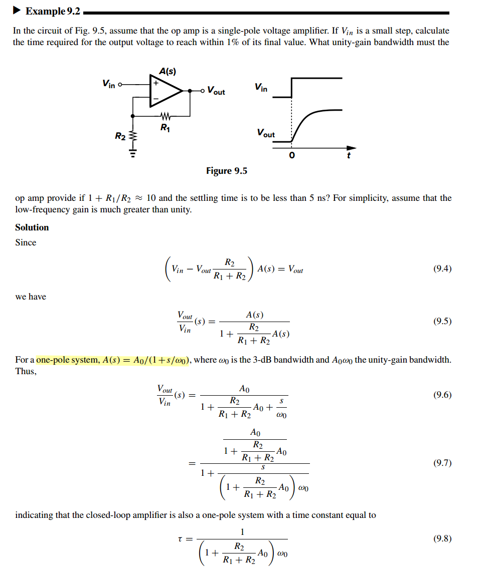
we have \[ \tau \approx \left(1 + \frac{R_1}{R_2}\right)\frac{1}{A_0\omega_0}= \frac{1}{\beta \omega_\text{ugb}} \]
Two Poles
with open-loop transfer function \(A_{OL}=\frac{A_0}{(1+s/\omega_1)(1+s/\omega_2)}\) and assuming \(\omega_1\) is dominant pole, then yield closed-loop transfer function
\[\begin{align} A_{CL}(s) &= \frac{\frac{A_0}{(1+s/\omega_1)(1+s/\omega_2)}}{1+\beta \frac{A_0} {(1+s/\omega_1)(1+s/\omega_2)}} \\ &= \frac{A_0}{1+A_0 \beta}\frac{1}{\frac{s^2}{\omega_1\omega_2(1+A_0\beta)}+\frac{1/\omega_1+1/\omega_2}{1+A_0\beta}s+1} \\ &\approx \frac{A_0}{1+A_0 \beta}\frac{1}{\frac{s^2}{\omega_u\omega_2}+\frac{1}{\omega_u}s+1} \\ &= \frac{A_0}{1+A_0 \beta}\frac{\omega_u\omega_2}{s^2+\omega_2s+\omega_u\omega_2} \end{align}\]
That is \(\omega_n = \sqrt{\omega_u\omega_2}\), \(\zeta = \frac{1}{2}\sqrt{\frac{\omega_2}{\omega_u}}\) , where \(\omega_u\approx \beta A_0 \omega_1\) is the unity gain bandwidth
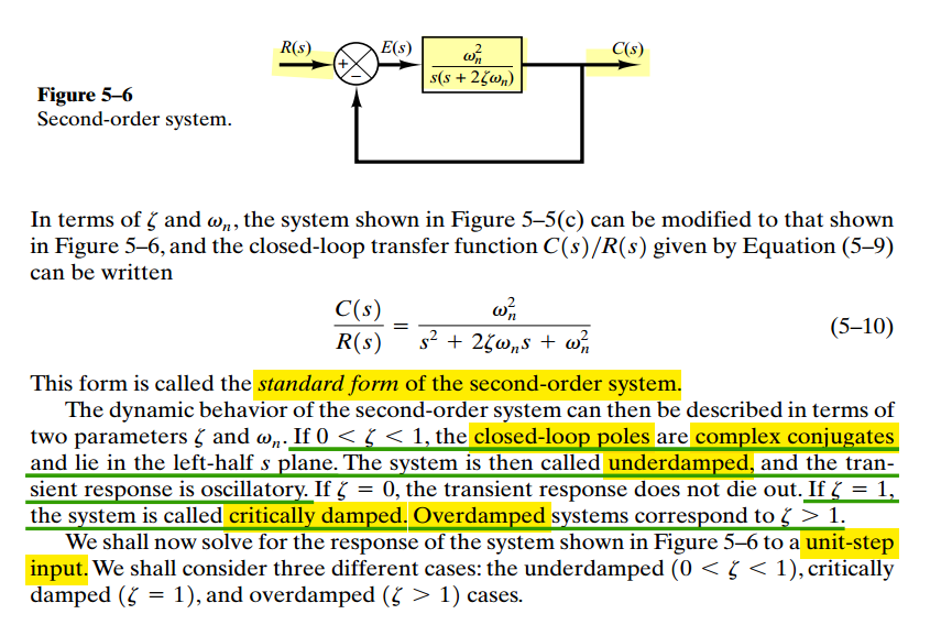
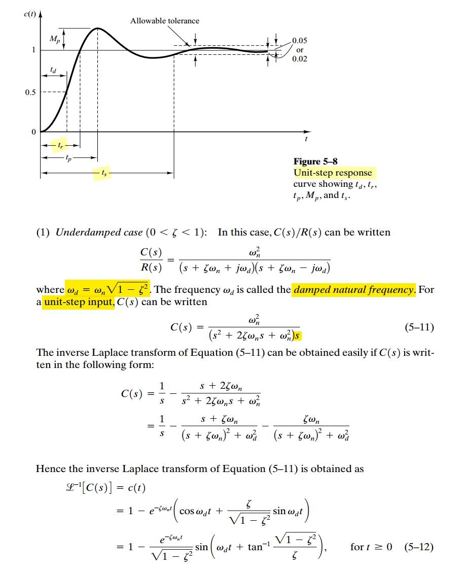
Rise Time (0% to 100% )
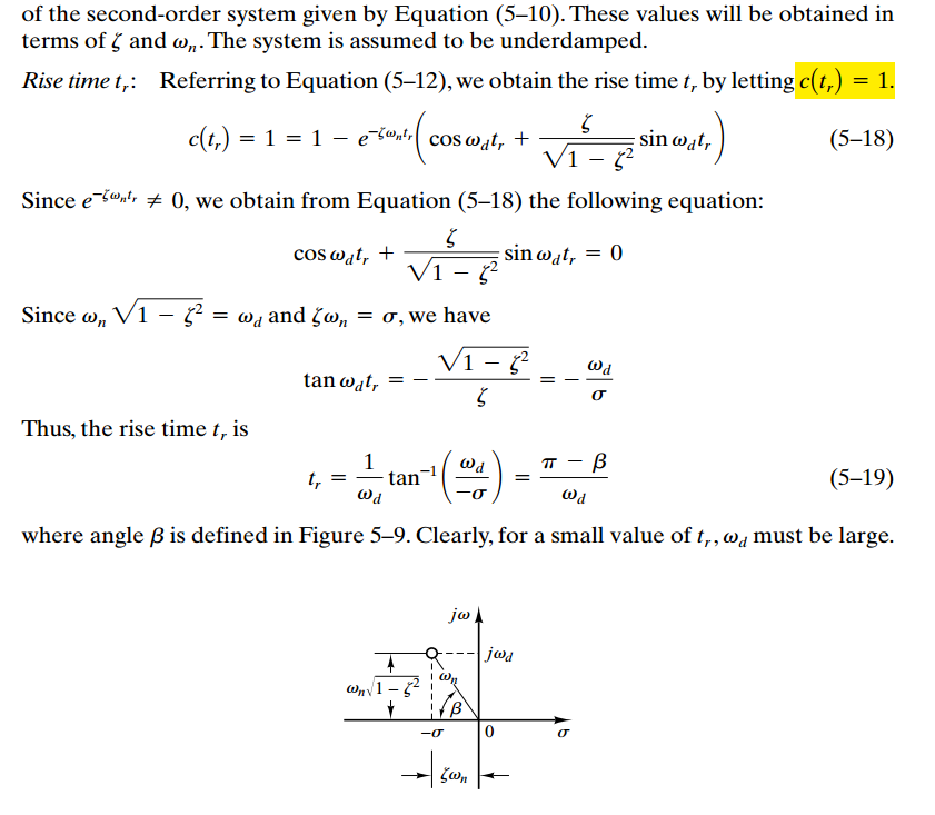
\[ t_r = \frac{\pi - \beta}{\omega_d}=\frac{\pi - \arctan\frac{\omega_n\sqrt{1-\zeta^2}}{\zeta\omega_n}}{\omega_n\sqrt{1-\zeta^2}}\approx\frac{\pi - \arctan\frac{\sqrt{1-\zeta^2}}{\zeta}}{\sqrt{\omega_u\omega_2}\sqrt{1-\zeta^2}}=\frac{\pi - \arctan\frac{\sqrt{1-\zeta^2}}{\zeta}}{\omega_u\sqrt{k(1-\zeta^2)}} \] where \(k = \frac{\omega_2}{\omega_u}\), is the function of PM
| PM | \(45^o\) | \(60^o\) | \(70^o\) |
|---|---|---|---|
| \(k\) | 1 | 1.73 | 2.75 |
| \(\zeta\) | 0.42 | 0.61 | 0.80 |
| \(t_r\) | \(\frac{2.2}{\omega_u}\) | \(\frac{2.14}{\omega_u}\) | \(\frac{2.53}{\omega_u}\) |
1 | PM = 70; |
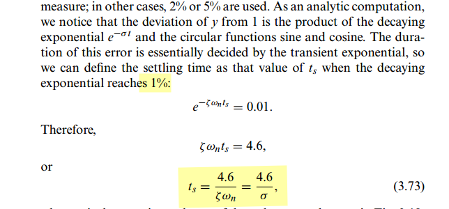
Settling Time
Gene F. Franklin, Feedback Control of Dynamic Systems, 8th Edition
As we know \[ \zeta \omega_n=\frac{1}{2}\sqrt{\frac{\omega_2}{\omega_u}}\cdot \sqrt{\omega_u\omega_2}=\frac{1}{2}\omega_2 \]
Then \[ t_s = \frac{9.2}{\omega_2} \]
For \(\text{PM}=70^o\), \(\omega_2 = 2.75\omega_u\), that is \[ t_s \approx \frac{3.35}{\omega_u} \]
For \(\text{PM}=45^o\), \(\omega_2 = \omega_u\), that is \[ t_s \approx \frac{9.2}{\omega_u} \]
Above equation is valid only for underdamped, \(\zeta=\frac{1}{2}\sqrt{\frac{\omega_2}{\omega_u}}\lt 1\), that is \(\omega_2\lt 4\omega_u\)
2 Stage RC filter
High Pass Filter
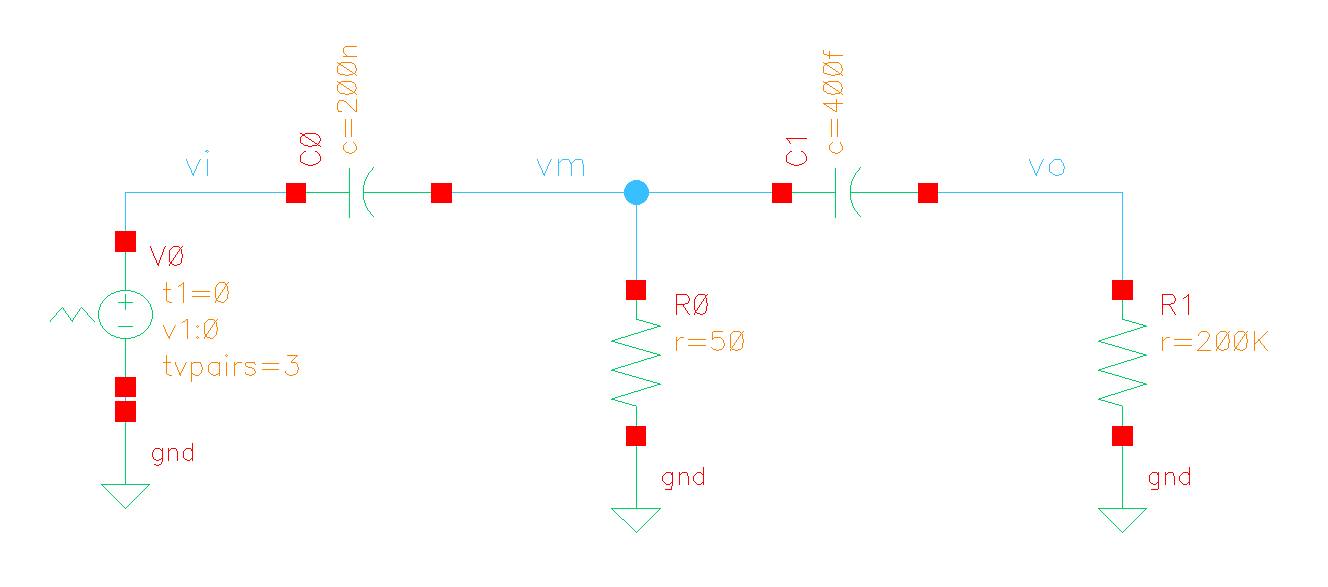
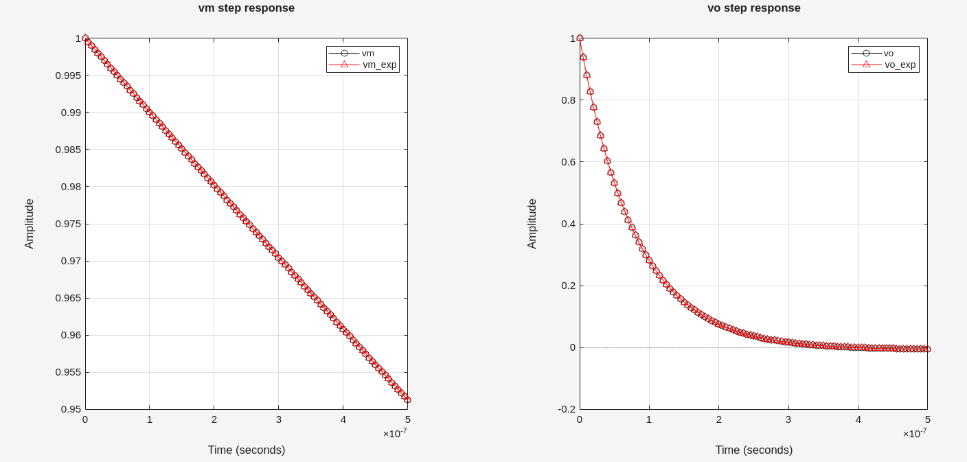
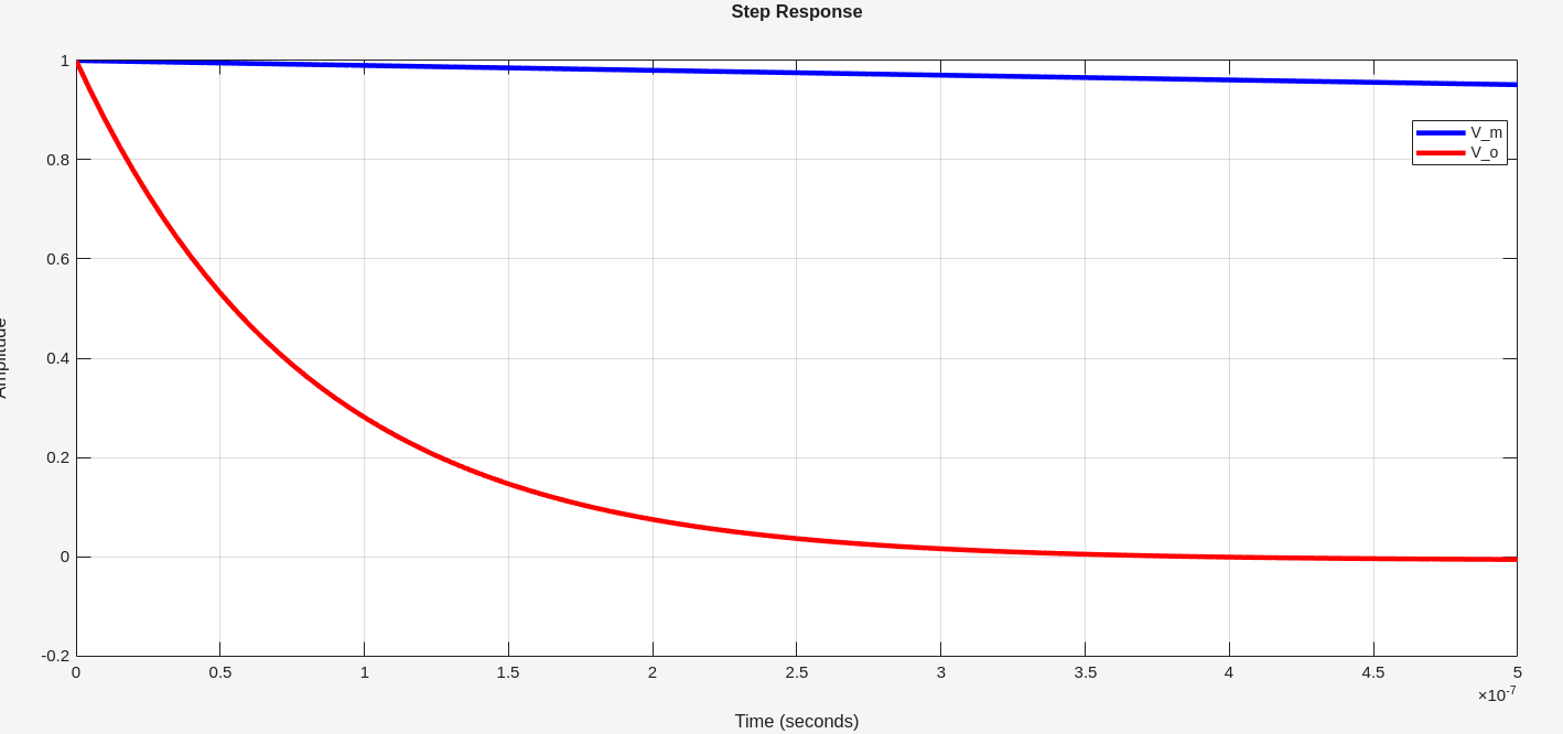
Since \(1/sC_1+R_1 \gg R_0\) \[ \frac{V_m}{V_i}(s) \approx \frac{R_0}{R_0 + 1/sC_0} = \frac{sR_0C_0}{1+sR_0C_0} \] step response of \(V_m\) \[ V_m(t) = e^{-t/R_0C_0} \] where \(\tau = R_0C_0\)
And \(V_o(s)\) can be expressed as \[\begin{align} \frac{V_o}{V_i}(s) & \approx \frac{sR_0C_0}{1+sR_0C_0} \cdot \frac{sR_1C_1}{1+sR_1C_1} \\ &= \frac{sR_0C_0R_1C_1}{R_0C_0-R_1C_1}\left(\frac{1}{1+sR_1C_1} - \frac{1}{1+sR_0C_0}\right) \end{align}\]
Then step response of \(Vo\) \[\begin{align} Vo(t) &= \frac{R_0C_0R_1C_1}{R_0C_0-R_1C_1} \left(\frac{1}{R_1C_1}e^{-t/R_1C_1} - \frac{1}{R_0C_0}e^{-t/R_0C_0}\right) \\ &= \frac{1}{R_0C_0-R_1C_1}\left(R_0C_0e^{-t/R_1C_1} - R_1C_1e^{-t/R_0C_0}\right) \\ &\approx \frac{1}{R_0C_0-R_1C_1}\left(R_0C_0e^{-t/R_1C_1} - R_1C_1\right) \end{align}\]
where \(\tau=R_1C_1\)
Partial-fraction Expansion
1 | syms C0 |
1 | >> partfrac(vm, s) |
\[\begin{align} V_m(s) &= 1 - \frac{s(C_1R_0+C_1R_1)+1}{C_0C_1R_0R_1s^2+(C_0R_0+C_1R_0+C_1R_1)s+1} \\ V_o(s) &= 1 - \frac{s(C_0R_0+C_1R_0+C_1R_1)+1}{C_0C_1R_0R_1s^2+(C_0R_0+C_1R_0+C_1R_1)s+1} \end{align}\]
1 | C0 = 200e-9; |
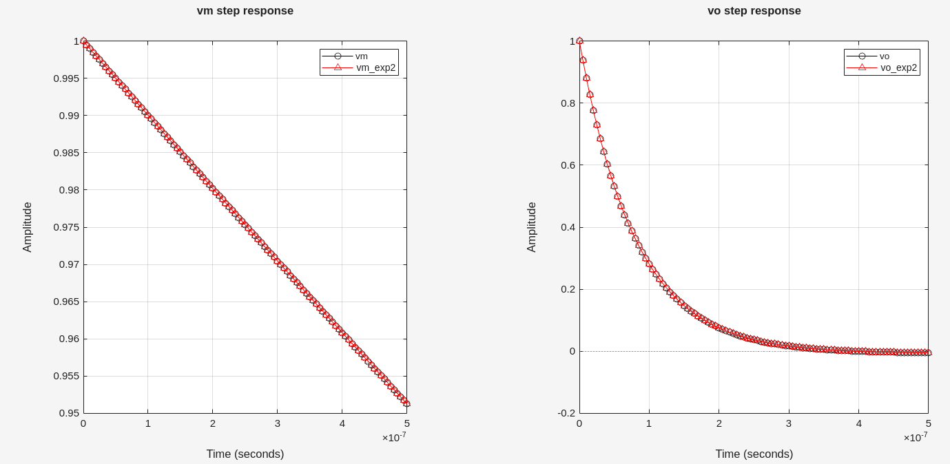
spectre vs matlab
1 | C0 = 200e-9; |
1 | >> vm |
Low Pass Filter
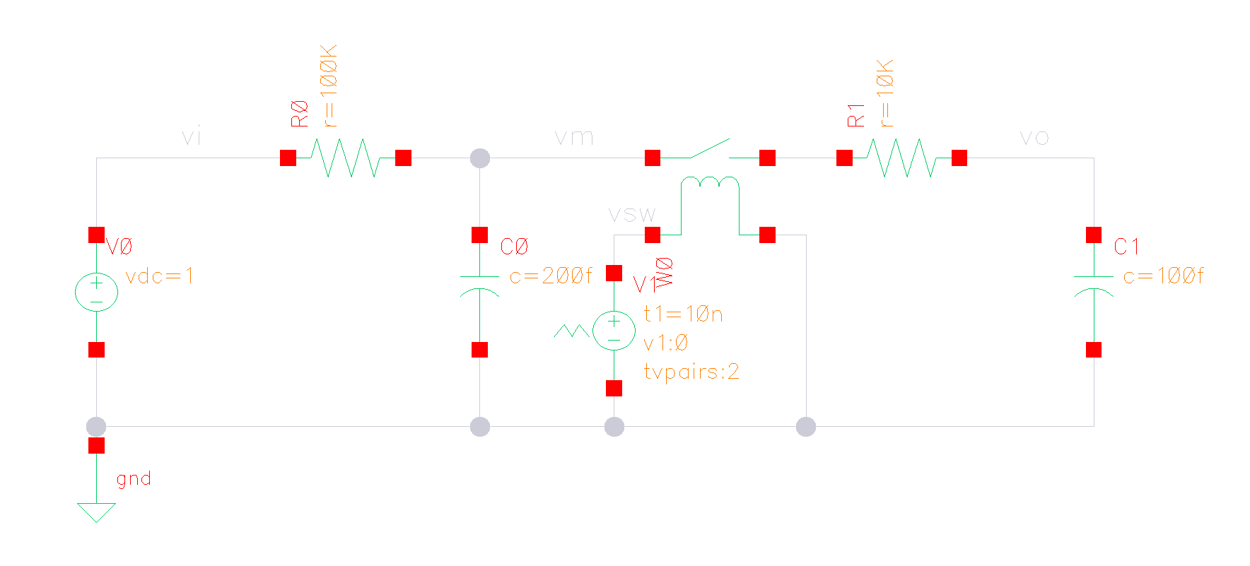
\[ \left\{ \begin{array}{cl} \frac{V_i - V_m}{R_0} &= C_0\frac{\mathrm{d}V_m}{\mathrm{d}t} + C_1\frac{\mathrm{d}V_o}{\mathrm{d}t} \\ \frac{V_m - V_o}{R_1} &= C_1\frac{\mathrm{d}V_o}{\mathrm{d}t} \\ V_m(t=0) &= 1 \\ V_o(t=0) &= 0 \end{array} \right. \]
Take into initial condition account \[ \frac{\mathrm{d}V_m}{\mathrm{d}t} \overset{\mathcal{L}}{\longrightarrow} sV_M-V_{m0} \] where \(V_{m0} = 1\)
\[\begin{align} V_O(s) &= \frac{V_I}{s^2R_0C_0R_1C_1+s(R_0C_0+R_1C_1+R_0C_1)+1} + \frac{V_{m0}R_0C_0}{s^2R_0C_0R_1C_1+s(R_0C_0+R_1C_1+R_0C_1)+1} \\ &\approx \frac{V_I}{s^2R_0C_0R_1C_1+sR_0(C_0+C_1)+1} + \frac{V_{m0}R_0C_0}{s^2R_0C_0R_1C_1+sR_0(C_0+C_1)+1} \\ &= \frac{V_I}{R_0(C_0+C_1)}\left(\frac{R_0(C_0+C_1)}{sR_0(C_0+C_1)+1} - \frac{R_1\frac{C_0C_1}{C_0+C_1}}{sR_1\frac{C_0C_1}{C_0+C_1}+1}\right) \\ &+ \frac{C_0}{C_0+C_1}\left(\frac{R_0(C_0+C_1)}{sR_0(C_0+C_1)+1} - \frac{R_1\frac{C_0C_1}{C_0+C_1}}{sR_1\frac{C_0C_1}{C_0+C_1}+1}\right) \end{align}\]
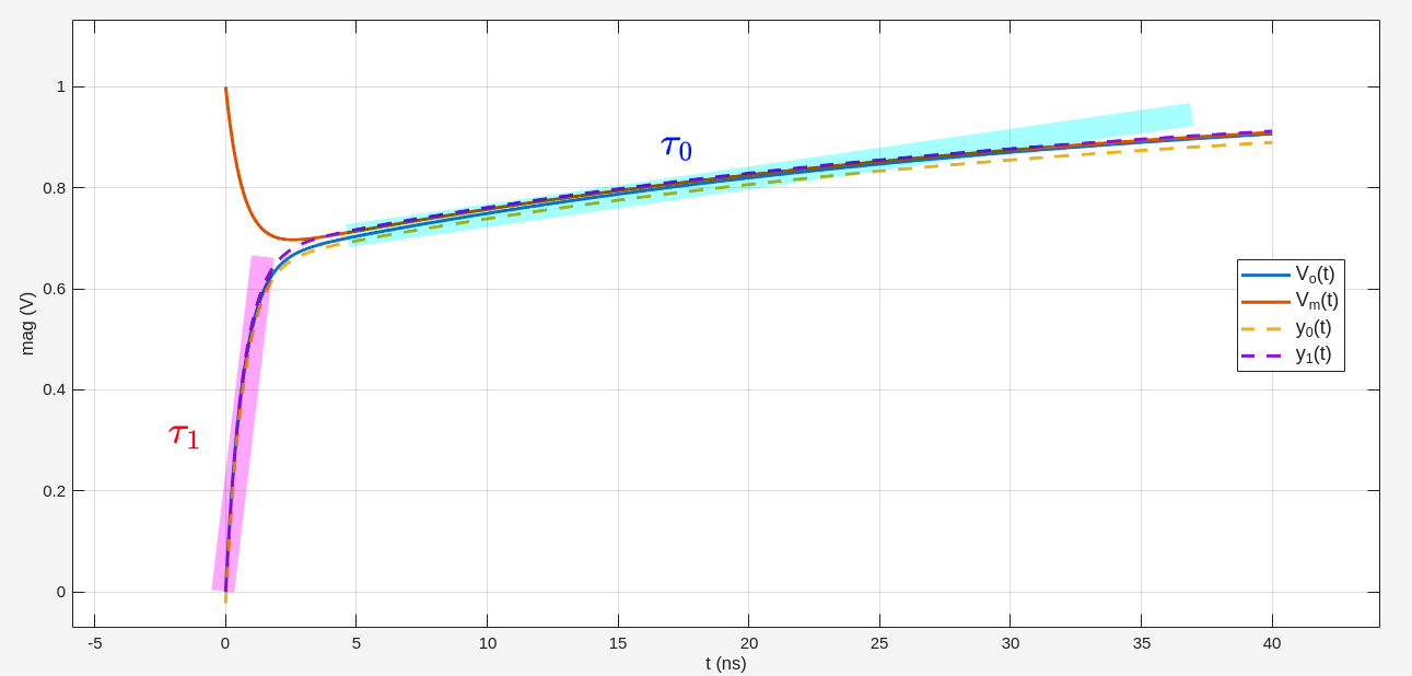
with \(V_I = \frac{1}{s}\), using inverse Laplace transform \[\begin{align} V_o(t) &= 1 - \frac{C_1}{C_0+C_1}e^{-t/\tau_0}-\frac{C_0}{C_0+C_1}e^{-t/\tau_1} - \frac{R_1C_0C_1}{R_0(C_0+C_1)^2} \tag{Eq.0} \\ &= 1 - \frac{C_1}{C_0+C_1}e^{-t/\tau_0}-\frac{C_0}{C_0+C_1}e^{-t/\tau_1} \tag{Eq.1} \end{align}\]
where
\[\begin{align} \tau_0 &= R_0(C_0+C_1) \\ \tau_1 &= R_1C_1\cdot \frac{C_0}{C_0+C_1} \end{align}\]
and \(\tau_0 \gg \tau_1\)
1 | R0 = 100e3; |
reference
Gene F. Franklin, J. David Powell, and Abbas Emami-Naeini. 2018. Feedback Control of Dynamic Systems (8th Edition) (8th. ed.). Pearson. [pdf]
Katsuhiko Ogata, Modern Control Engineering, 5th edition [pdf]
C. T. Chuang, "Analysis of the settling behavior of an operational amplifier," in IEEE Journal of Solid-State Circuits, vol. 17, no. 1, pp. 74-80, Feb. 1982 [https://sci-hub.se/10.1109/JSSC.1982.1051689]
Jason Sachs, Second-Order Systems, Part I: Boing!! [https://www.embeddedrelated.com/showarticle/671.php]