Noise Analysis
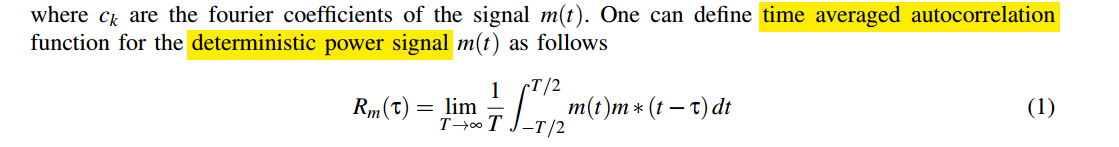
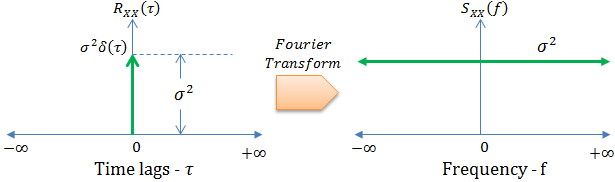
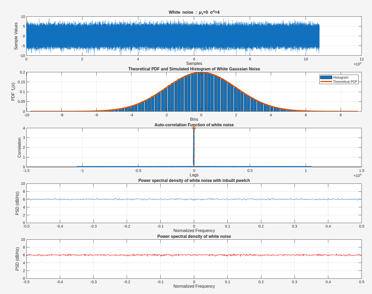
White noise
David Murray. Topic 6: Random Processes and Signals [slides notes]
Mathuranathan. White Noise : Simulation and Analysis using Matlab [https://www.gaussianwaves.com/2013/11/simulation-and-analysis-of-white-noise-in-matlab/]
1 | clear all; clc; close all; |
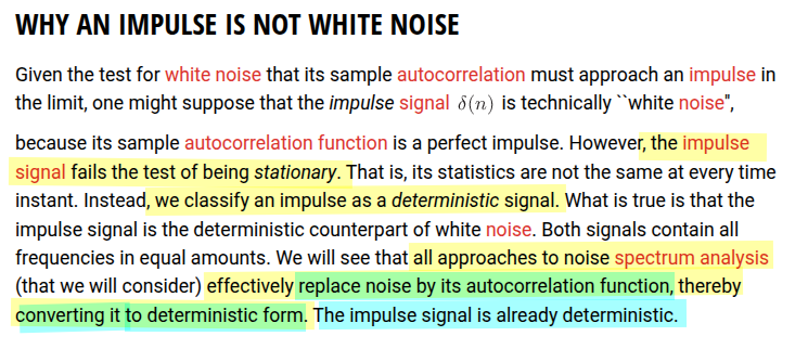
Julius Orion Smith III. Why an Impulse is Not White [https://www.dsprelated.com/freebooks/sasp/Why_Impulse_Not_White.html]
I.I.D. Noise
Independent and Identically Distributed
Kevin Zheng. The Frequency Domain Trap – Beware of Your AC Analysis [https://circuit-artists.com/the-frequency-domain-trap-beware-of-your-ac-analysis/]
Mathuranathan. White Noise : Simulation and Analysis using Matlab [https://www.gaussianwaves.com/2013/11/simulation-and-analysis-of-white-noise-in-matlab/]
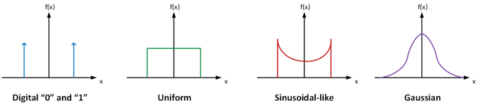
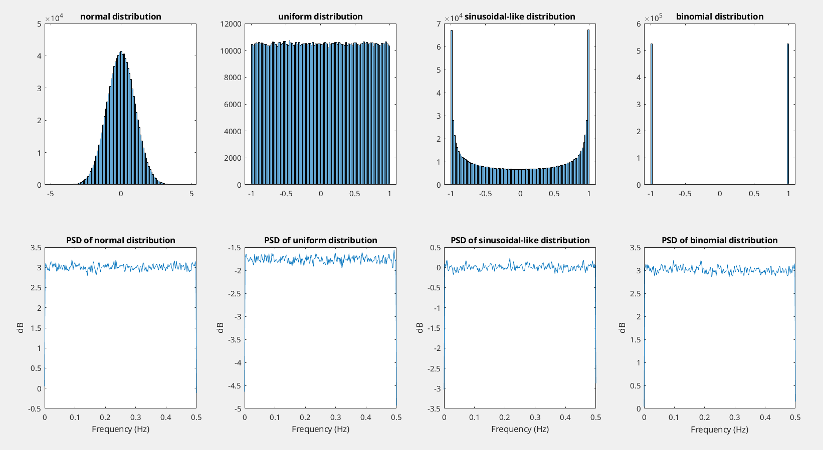
white noise doesn't mean it has a Gaussian/normal distribution
The only criteria for a (discrete) signal to be "white" is for each sample to be independently taken from the same probability distribution
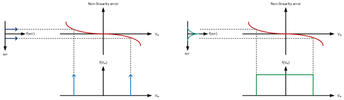
By understanding input signal's statistical nature, we can gather more insights about certain requirements for our circuits than just from frequency domain
1 | fs = 1; |
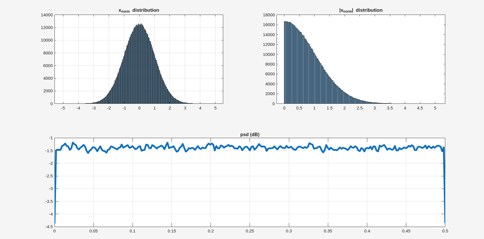
1 | val = randn(1, 2^20,1); |
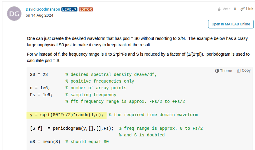
Additive White Gaussian Noise (AWGN)
Qasim Chaudhari. Additive White Gaussian Noise (AWGN) [https://wirelesspi.com/additive-white-gaussian-noise-awgn/]
Mathuranathan. Simulate additive white Gaussian noise (AWGN) channel [https://www.gaussianwaves.com/2015/06/how-to-generate-awgn-noise-in-matlaboctave-without-using-in-built-awgn-function/]
Does PSD (dBm/Hz) of white noise depend on sampling rate?. Does PSD (dBm/Hz) of white noise depend on sampling rate? [https://dsp.stackexchange.com/a/87654/59253]
Matthew Schubert. Colouring Noise - Generating coloured noise to simulate physical processes [https://blog.ioces.com/matt/posts/colouring-noise/]
\[ \text{PSD}_s = \frac{\sigma^2}{f_s} \space\space \text{for two-sided PSD} \space\space\space \text{or}\space\space\space =\frac{\sigma^2}{f_s/2}\space\space \text{for one-sided PSD} \]
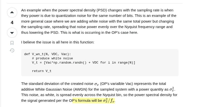
that total power will always be the same for any sampling rate used (as long as the histogram of those samples is still \(\sigma_x\)). Thus the power spectral density will be \(\sigma_x^2/f_s\).

How to generate white noise signal from a given PSD? [https://www.mathworks.com/matlabcentral/answers/1968-how-to-generate-white-noise-signal-from-a-given-psd#answer_1498849]
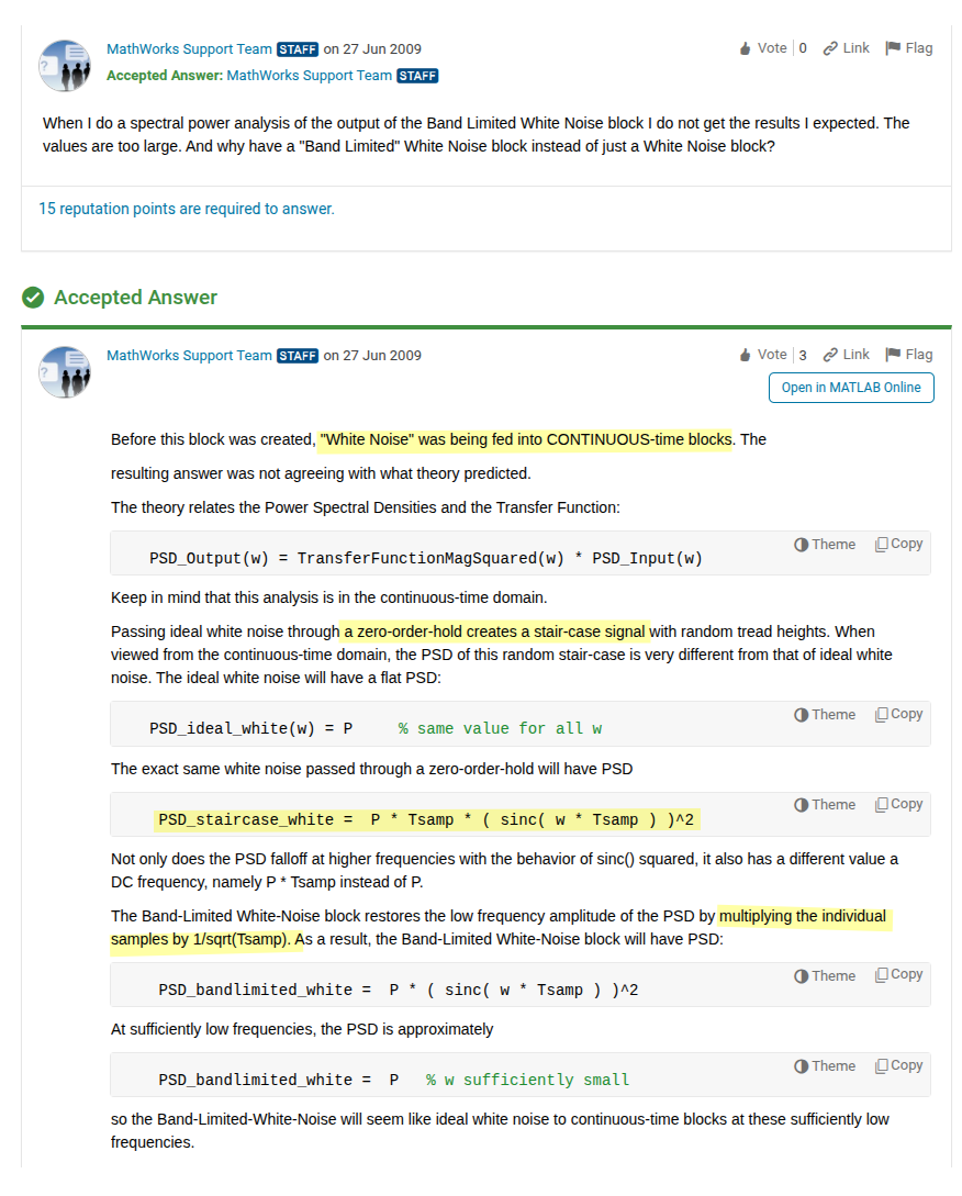
White noise in CONTINUOUS-time blocks
MathWorks Support Team. [https://www.mathworks.com/matlabcentral/answers/100763-why-have-a-band-limited-white-noise-generator-block-instead-of-just-a-white-noise-generator-block#answer_110112]

Colored Noise Generation
Allen B. Downey. Think DSP - Digital Signal Processing in Python [book repo]
Chembian Thambidurai, "Comparison Of Noise Power At Lowpass Filter Output" [link]
—, "On Noise Power At The Bandpass Filter Output" [link]
Steve Smith. An Interesting Fourier Transform - 1/f Noise [https://www.dsprelated.com/showarticle/40.php]
Mathuranathan. Generate correlated Gaussian sequence (colored noise) [https://www.gaussianwaves.com/2019/10/generating-correlated-gaussian-sequences/]
Jeruchim et., al, Simulation of communication systems – modeling, methodology, and techniques, second edition, Kluwer academic publishers, 2002
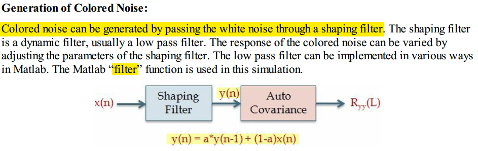
Two methods to generate colored Gaussian noise for given mean and PSD shape
- Spectral Factorization Method
- Auto-Regressive (AR) Model
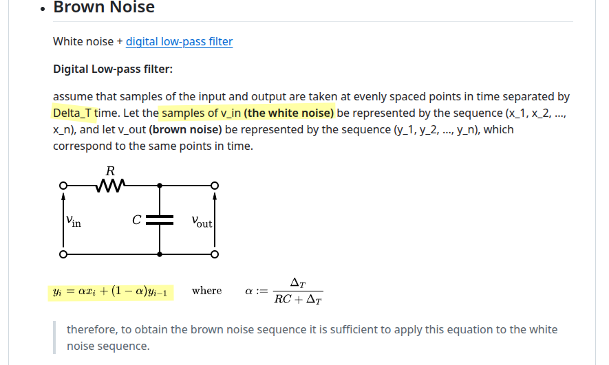
Filtering in Time domain
Alessandro Cudazzo. noise generator developed in C99 (white, brown) [https://github.com/alessandrocuda/noise_generator]
with Derivatives approximation, \(H_p(s) = \frac{1}{s\tau + 1} \to H_p(z)=\frac{\alpha}{1 +(\alpha -1)z^{-1}}\), where \(\alpha = \frac{T}{\tau+T}\)
1 | get_bnoise(){ |
1 | %Colored Noise Generation |
Julius Orion Smith III. Spectral Audio Signal Processing [https://www.dsprelated.com/freebooks/sasp/Filtered_White_Noise.html]
Example: Synthesis of 1/F Noise (Pink Noise)
1 | Nx = 2^16; % number of samples to synthesize |
Filtering in Frequency domain
Matthew Schubert. Colouring Noise - Generating coloured noise to simulate physical processes [https://blog.ioces.com/matt/posts/colouring-noise/] [https://gist.github.com/m-schubert/45c562146c6607b8990f1e8f34ff87b0]
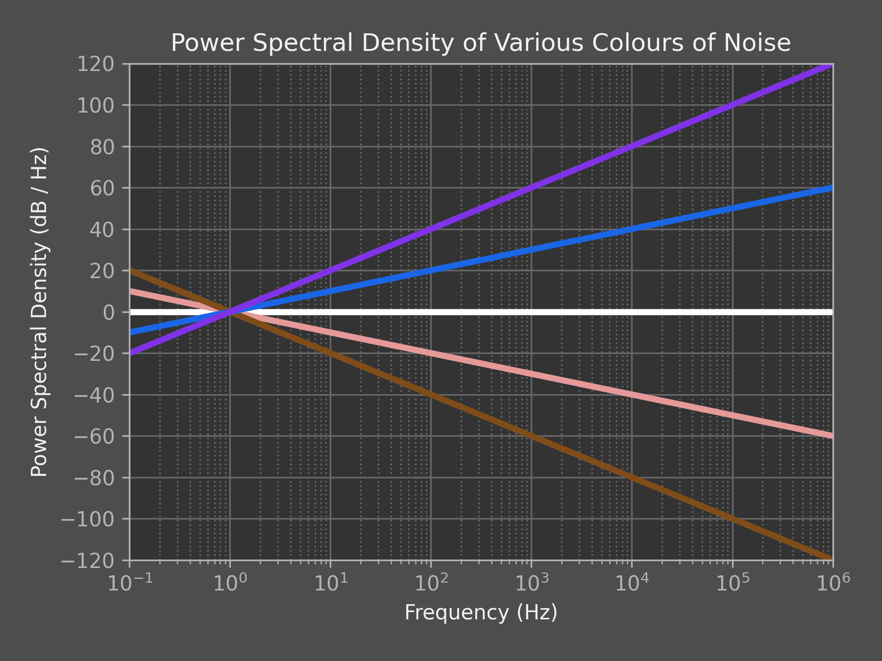
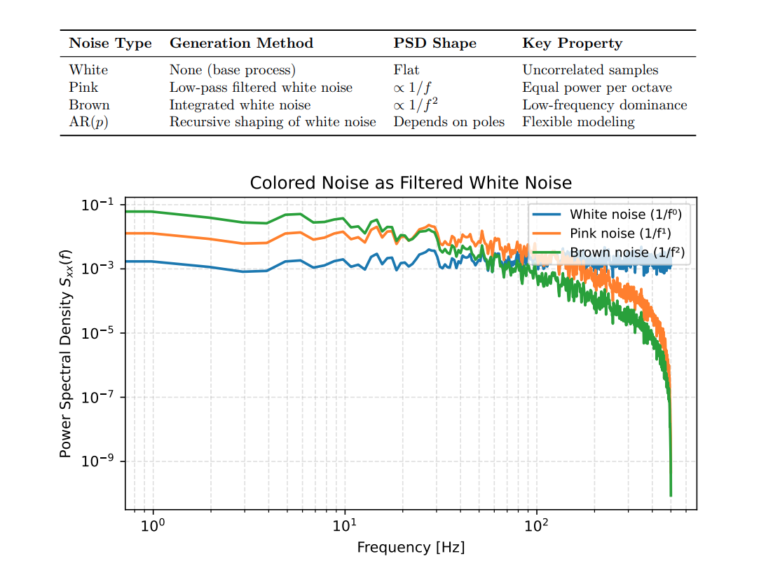
White, Pink \(1/f\), Brownian \(1/f^2\), Blue \(f\), Violet \(f^2\)
The process of generating coloured noise is relatively simple:
- Start with a representation of white noise signal in the frequency domain
- Shape the signal in the frequency domain according to the PSD you'd like to achieve
- Take the inverse Fourier transform of the shaped signal
Sampling shaping transfer function (not scaled by \(1/T_s\)) make sense in time domain convolution between sampled noise and sampled impulse response of filter
AR(N) Model Method
Generate color noise using Auto-Regressive (AR) model [https://www.gaussianwaves.com/2019/12/color-noise-generation-using-auto-regressive-ar-model-power-law-noises/]
Konstantinos Chatzilygeroudis. Lecture 9 & 10: Noise Models & Linear Filters [notes, slides]
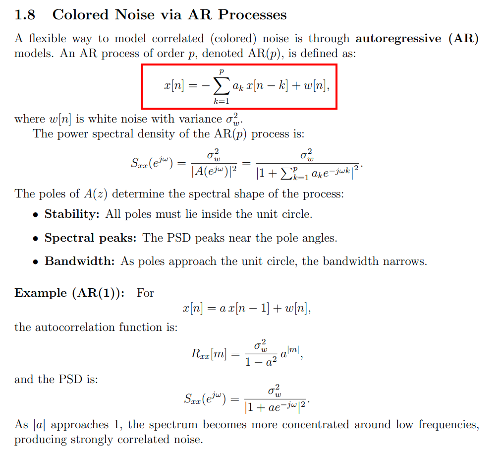
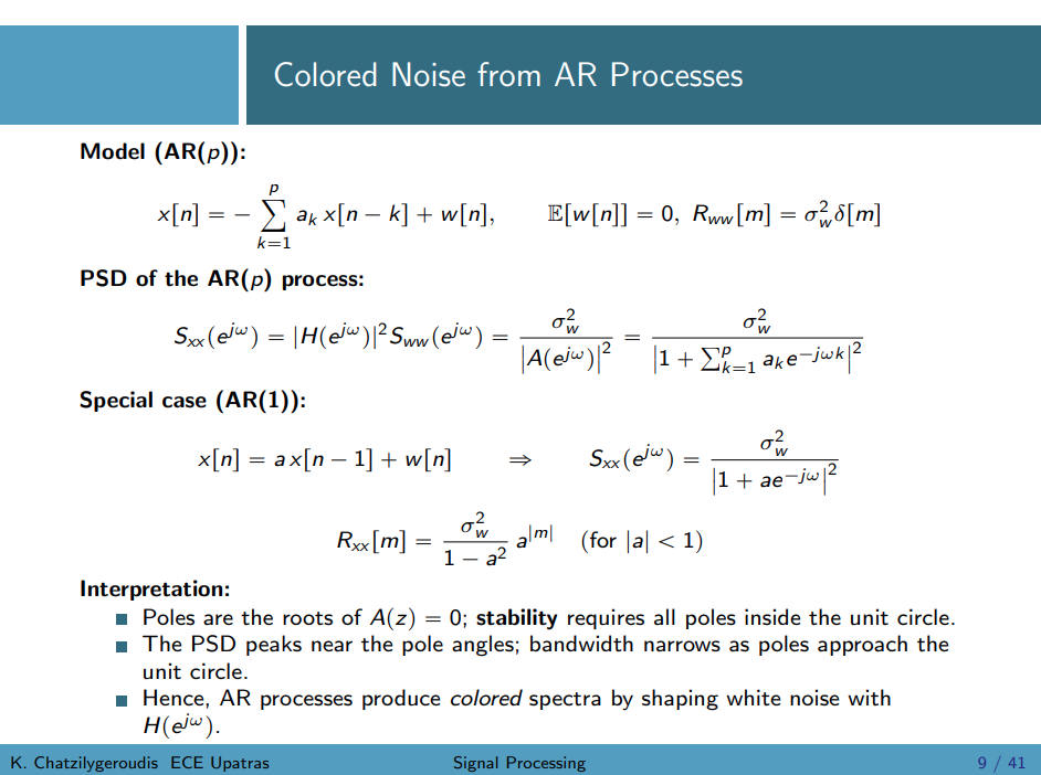
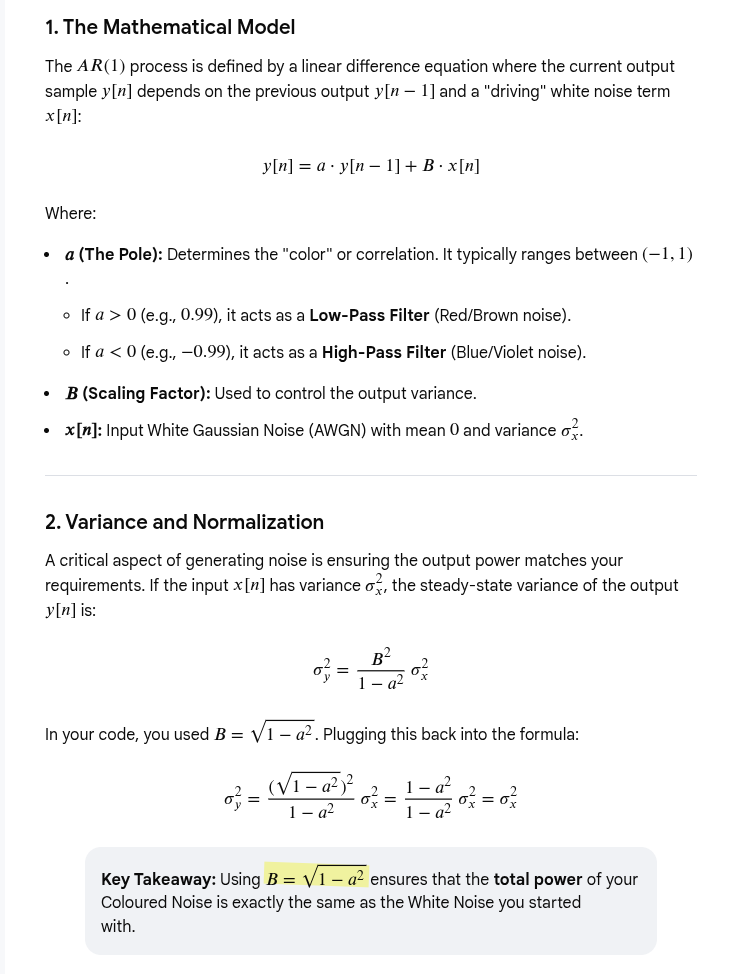
Autoregressive (AR) modeling in signal processing represents a signal as a linear combination of its own previous values plus a white noise error term, effectively acting as an all-pole IIR filter
Google AI Mode [https://share.google/aimode/QAuvWdwJFng54cYZo]
1 | % https://github.com/vineel49/colored_noise/blob/master/RUN_ME.m |
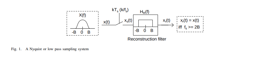
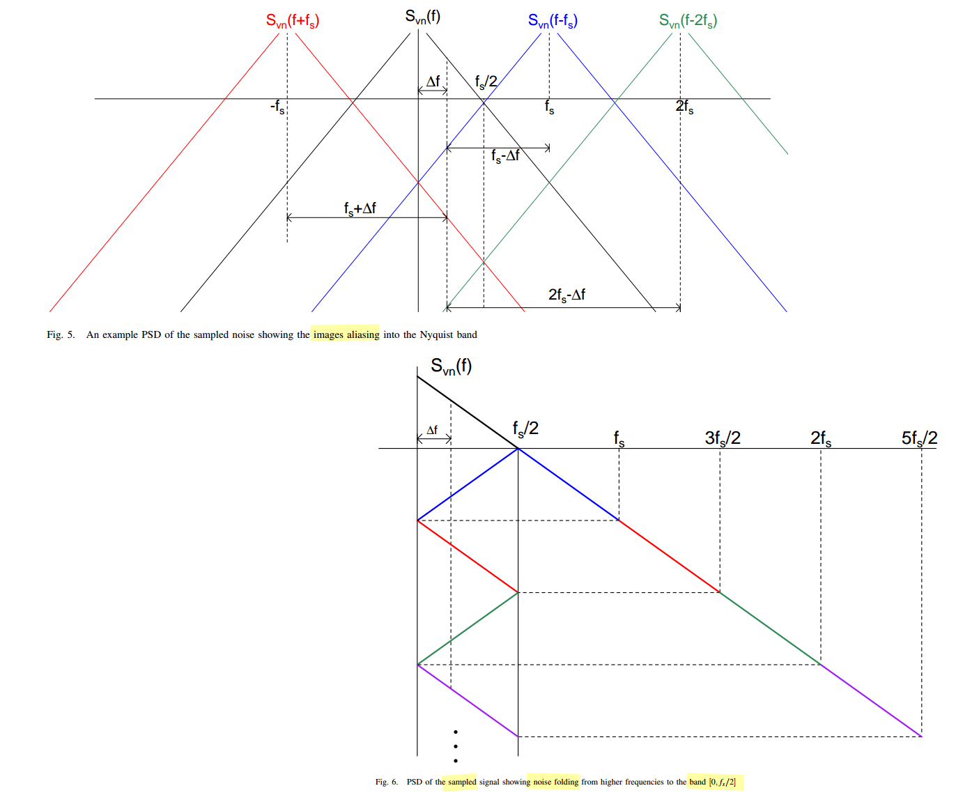
sampling bandlimited white noise
The aliasing of the noise, or noise folding, plays an important role in switched-capacitor as it does in all switched-capacitor filters
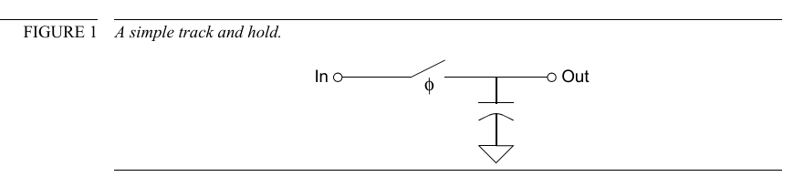
Assume for the moment that the switch is always closed (that there is no hold phase), the single-sided noise density would be
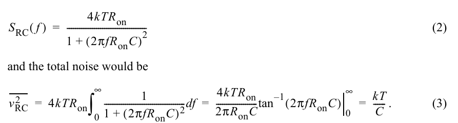
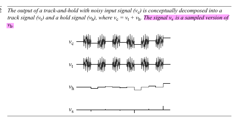
\(v_s[n]\) is the sampled version of \(v_{RC}(t)\), i.e. \(v_s[n]= v_{RC}(nT_C)\) \[ S_s(e^{j\omega}) = \frac{1}{T_C} \sum_{k=-\infty}^{\infty}S_{RC}(j(\frac{\omega}{T_C}-\frac{2\pi k}{T_C})) \cdot d\omega \] where \(\omega \in [-\pi, \pi]\), furthermore \(\frac{d\omega}{T_C}= d\Omega\) \[ S_s(j\Omega) = \sum_{k=-\infty}^{\infty}S_{RC}(j(\Omega-k\Omega_s)) \cdot d\Omega \]

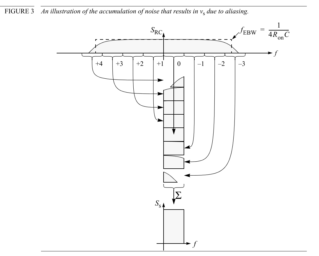
The noise in \(S_{RC}\) is a stationary process and so is uncorrelated over \(f\) allowing the \(N\) rectangles to be combined by simply summing their noise powers
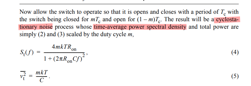
where \(m\) is the duty cycle
Kundert, Ken. (2006). Simulating Switched-Capacitor Filters with SpectreRF [https://designers-guide.org/analysis/sc-filters.pdf]
Pavan, Schreier and Temes, "Understanding Delta-Sigma Data Converters, Second Edition" ISBN 978-1-119-25827-8
Tania Khanna, ESE568 Fall 2019, Mixed Signal Circuit Design and Modeling URL: https://www.seas.upenn.edu/~ese568/fall2019/
Matt Pharr, Wenzel Jakob, and Greg Humphreys. 2016. Physically Based Rendering: From Theory to Implementation (3rd. ed.). Morgan Kaufmann Publishers Inc., San Francisco, CA, USA.
R. Gregorian and G. C. Temes. Analog MOS Integrated Circuits for Signal Processing. Wiley-Interscience, 1986
Trevor Caldwell, Lecture 9 Noise in Switched-Capacitor Circuits [http://individual.utoronto.ca/trevorcaldwell/course/NoiseSC.pdf]
Christian-Charles Enz. High precision CMOS micropower amplifiers [pdf]
Below analysis focusing on sampled noise
Boris Murmann. Noise Analysis in Switched-Capacitor Circuits, ISSCC 2011 / tutorials [slides, transcript]
—. EE315A VLSI Signal Conditioning Circuits [pdf]
—. EE315B VLSI Data Conversion Circuits, Autumn 2013 [pdf]
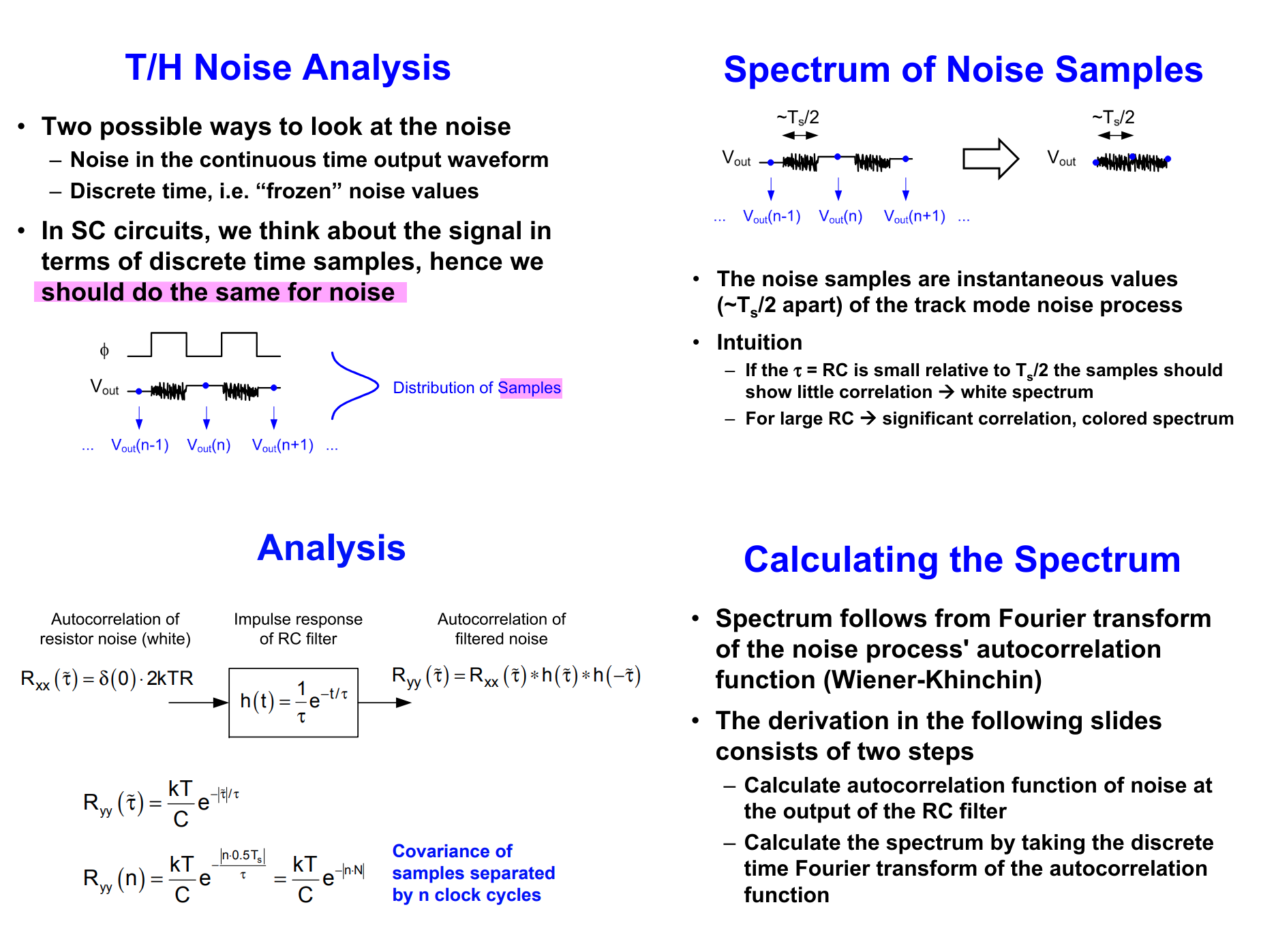
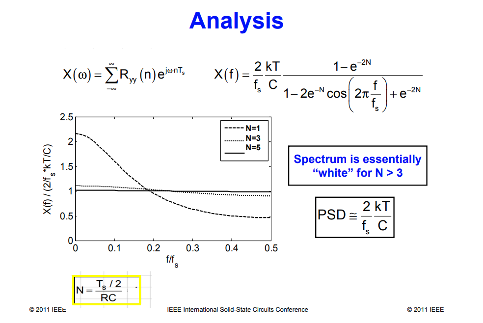
- Calculate autocorrelation function of noise at the output of the RC filter
- Calculate the spectrum by taking the discrete time Fourier transform of the autocorrelation function
Bernhard E. Boser . Advanced Analog Integrated Circuits Switched Capacitor Gain Stages [https://people.eecs.berkeley.edu/~boser/courses/240B/lectures/M05%20SC%20Gain%20Stages.pdf]
impulse sampling noise
Chembian Thambidurai, "Noise, Sampling and Zeta Functions" [link]
A random signal \(v_n(t)\) is sampled using an ideal impulse sampler
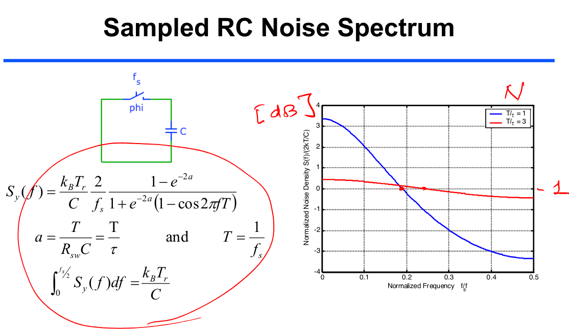
Sampling coloured noise
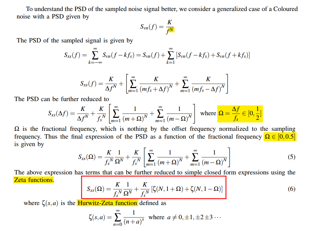
converging PSD
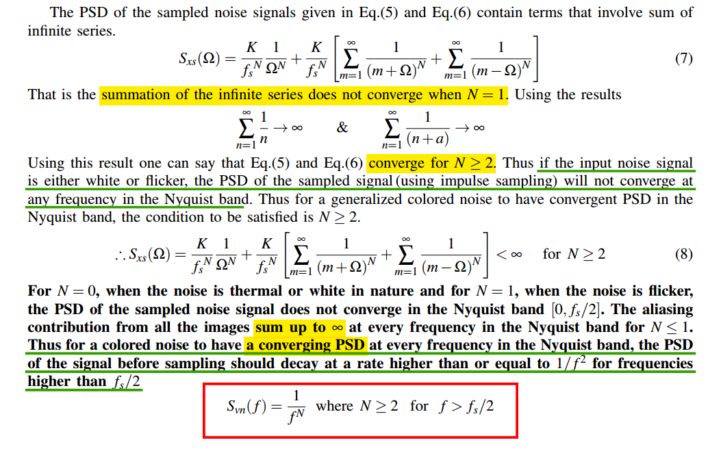
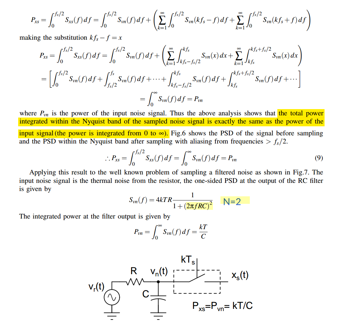
integrated power of the sampled signal in the Nyquist band
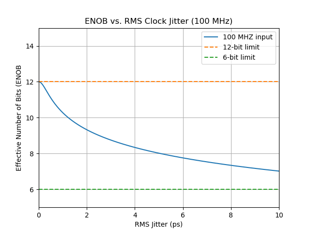
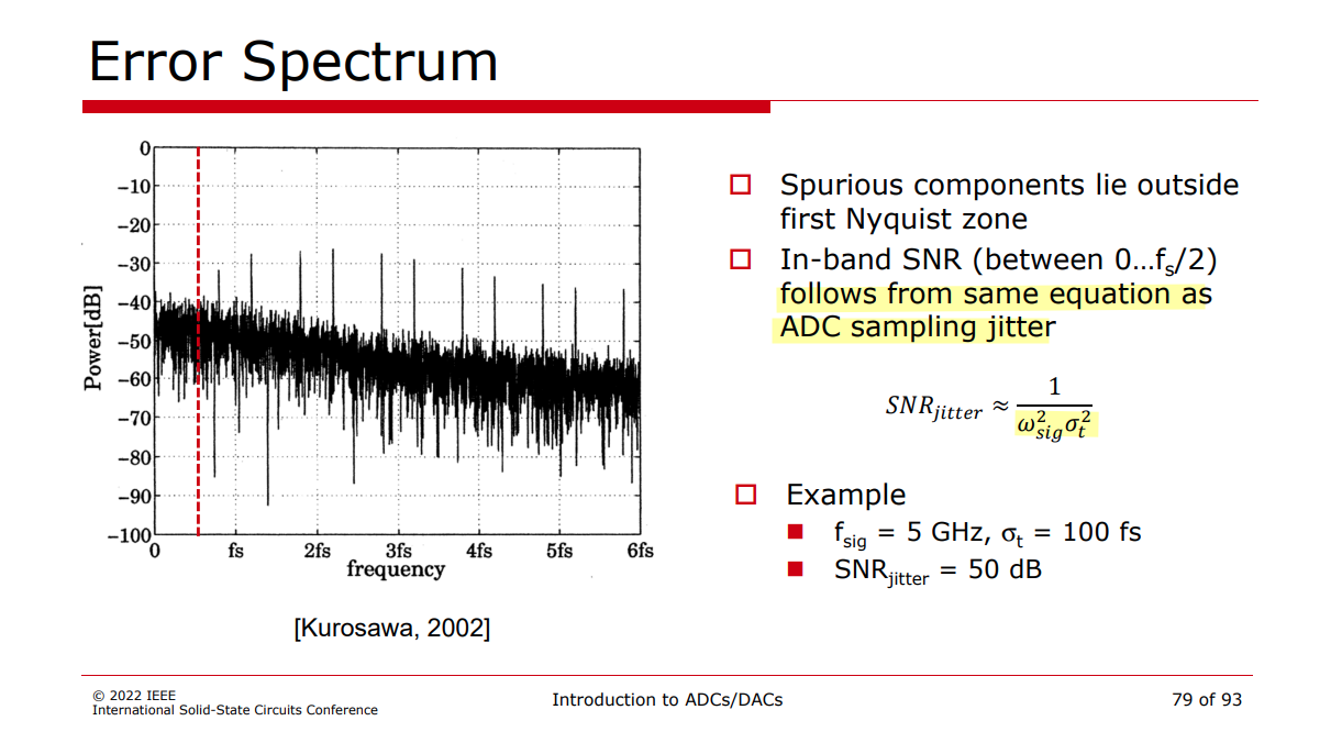
ADC SNR & clock jitter
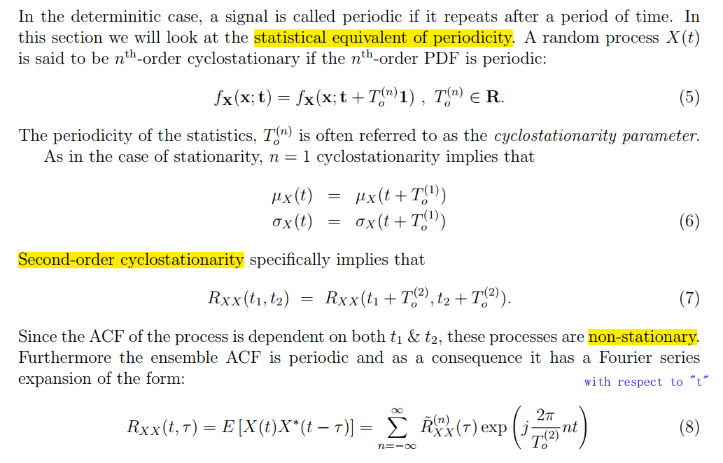
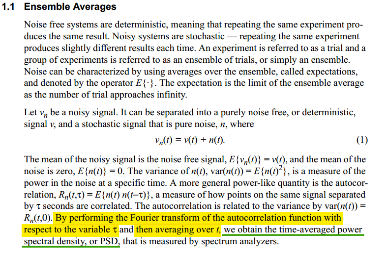
cyclostationary random process
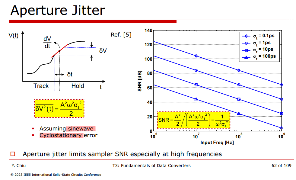
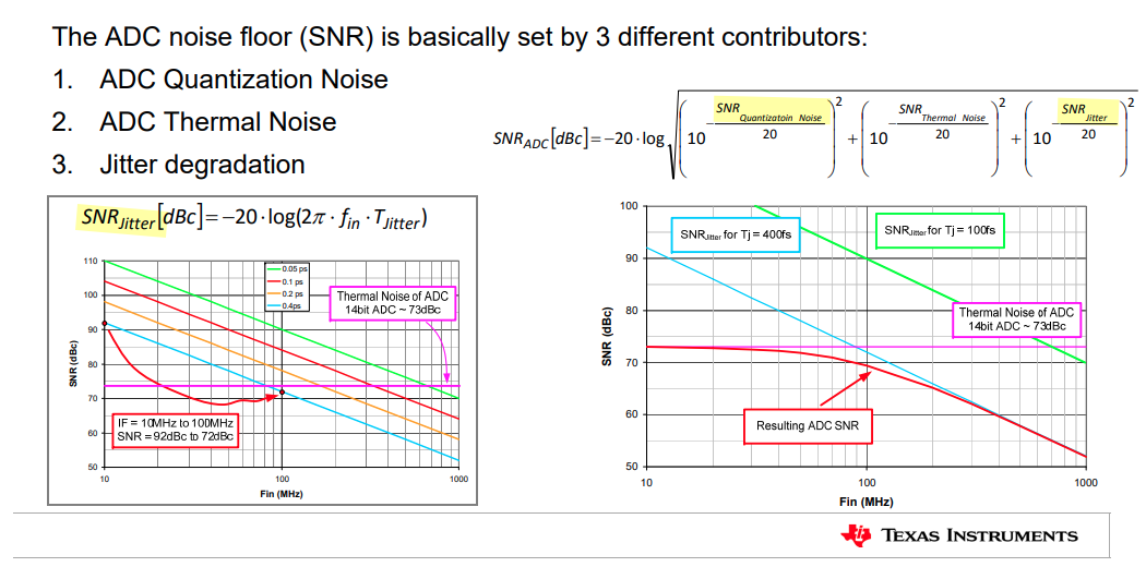
\[\begin{align} \text{SNR}_\text{ADC}[\text{dB}] &= -20\cdot \log \sqrt{\left(10^{-\frac{\text{SNR}_\text{Quantization Noise}}{20}}\right)^2 + \left(10^{-\frac{\text{SNR}_\text{Jitter}}{20}}\right)^2} \\ &= -10\cdot \log \left(\left(10^{-\frac{\text{SNR}_\text{Quantization Noise}}{20}}\right)^2 + \left(10^{-\frac{\text{SNR}_\text{Jitter}}{20}}\right)^2\right) \\ &= -10\cdot \log \left(\left(10^{-\frac{10\log(\frac{3\times2^{2N}}{2})}{20}}\right)^2 + \left(10^{-\frac{-20\log{(2\pi f_\text{in}\sigma_\text{jitter})}}{20}}\right)^2\right) \\ &= -10\cdot \log \left( \frac{2}{3\times 2^{2N}} + (2\pi f_\text{in}\sigma_\text{jitter})^2 \right) \end{align}\]
Ayça Akkaya, "High-Speed ADC Design and Optimization for Wireline Links" [https://infoscience.epfl.ch/server/api/core/bitstreams/96216029-c2ff-48e5-a675-609c1e26289c/content]
CC Chen, Why Absolute Jitter Matters for ADCs & DACs? [https://youtu.be/jBgDDFFDq30]
Thomas Neu, TIPL 4704. Jitter vs SNR for ADCs [https://www.ti.com/content/dam/videos/external-videos/en-us/2/3816841626001/5529003238001.mp4/subassets/TIPL-4704-Jitter-vs-SNR.pdf]
1 | import numpy as np |
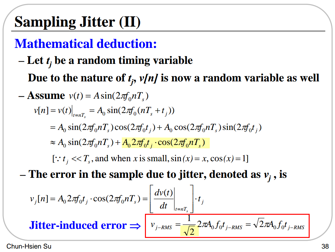
Chun-Hsien Su (蘇純賢). Design of Oversampled Sigma-Delta Data Converters. July, 2006 [pdf]
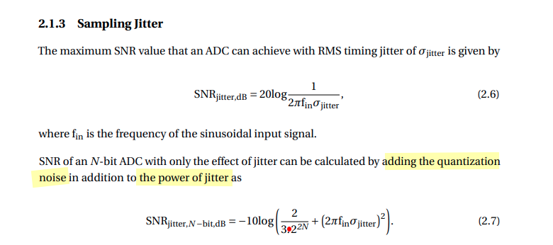
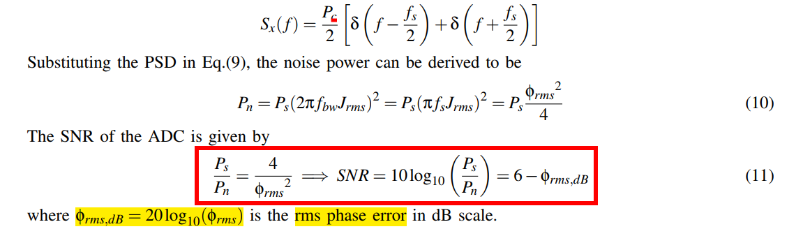
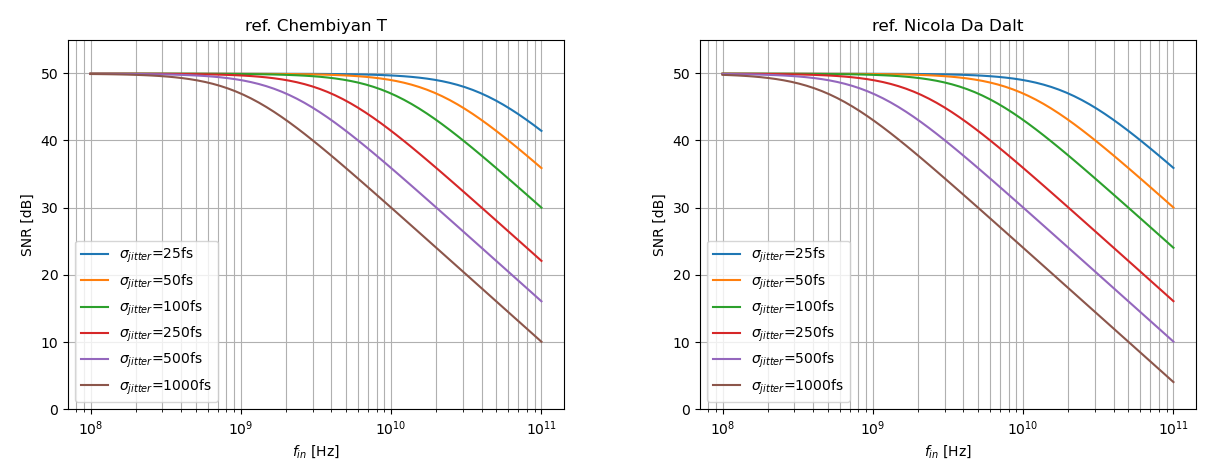
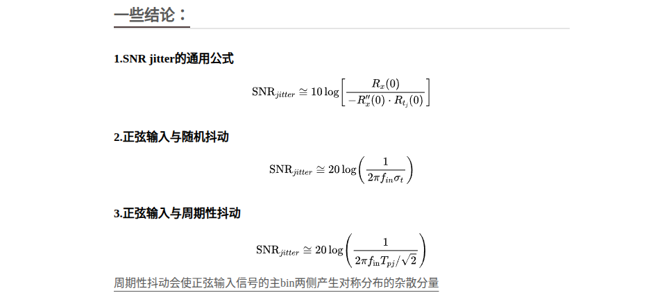
Chembian Thambidurai, "SNR of an ADC in the presence of clock jitter" [https://www.linkedin.com/posts/chembiyan-t-0b34b910_adcsnrjitter-activity-7171178121021304833-f2Wd/]
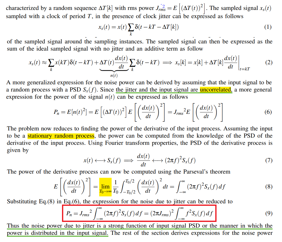
Unlike the quantization noise and the thermal noise, the impact of the clock jitter on the ADC performance depends on the input signal properties like its PSD
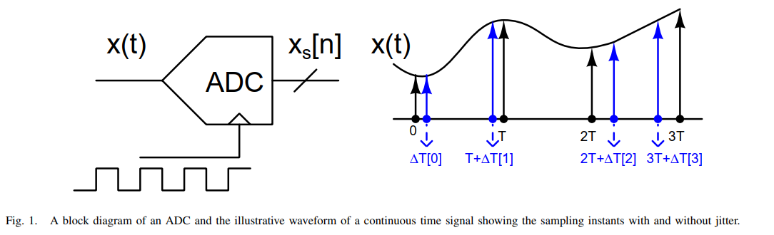
The error between the ideal sampled signal and the sampling with clock jitter can be treated as noise and it results in the degradation of the SNR of the ADC
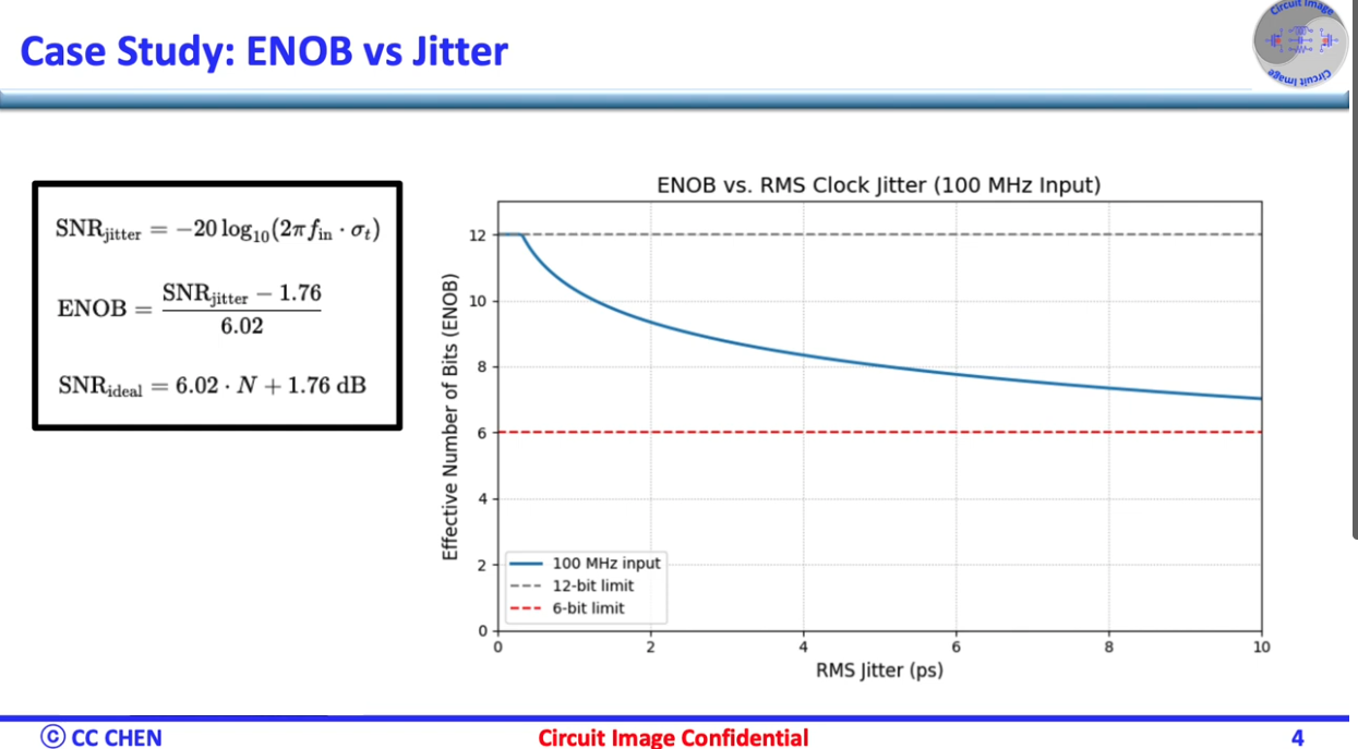
For sinusoid input:
1 | import numpy as np |
K. Tyagi and B. Razavi, "Performance Bounds of ADC-Based Receivers Due to Clock Jitter," in IEEE Transactions on Circuits and Systems II: Express Briefs, vol. 70, no. 5, pp. 1749-1753, May 2023 [https://www.seas.ucla.edu/brweb/papers/Journals/KT_TCAS_2023.pdf]
N. Da Dalt, M. Harteneck, C. Sandner and A. Wiesbauer, "On the jitter requirements of the sampling clock for analog-to-digital converters," in IEEE Transactions on Circuits and Systems I: Fundamental Theory and Applications, vol. 49, no. 9, pp. 1354-1360, Sept. 2002 [https://sci-hub.se/10.1109/TCSI.2002.802353]
M. Shinagawa, Y. Akazawa and T. Wakimoto, "Jitter analysis of high-speed sampling systems," in IEEE Journal of Solid-State Circuits, vol. 25, no. 1, pp. 220-224, Feb. 1990 [https://sci-hub.se/10.1109/4.50307]
Ayça Akkaya, "High-Speed ADC Design and Optimization for Wireline Links" [https://infoscience.epfl.ch/server/api/core/bitstreams/96216029-c2ff-48e5-a675-609c1e26289c/content]

待学芯. ADC量化结果反推采样时钟抖动(Jitter) [https://mp.weixin.qq.com/s/55xfVQMe_N8zUGpI8ZvmsQ]
—. 关于时钟抖动(Jitter)与ADC的一些讨论 [https://mp.weixin.qq.com/s/GW1keHhfq7zrd036lyG0CQ]
DAC SNR & clock jitter
ampling Jitter Effects for ADC/DAC
- In both DAC or ADC cases, doubling the timing jitter doubles the noise level
- Also, doubling the frequency or amplitude doubles the jitter induced noise - SNR is not improved
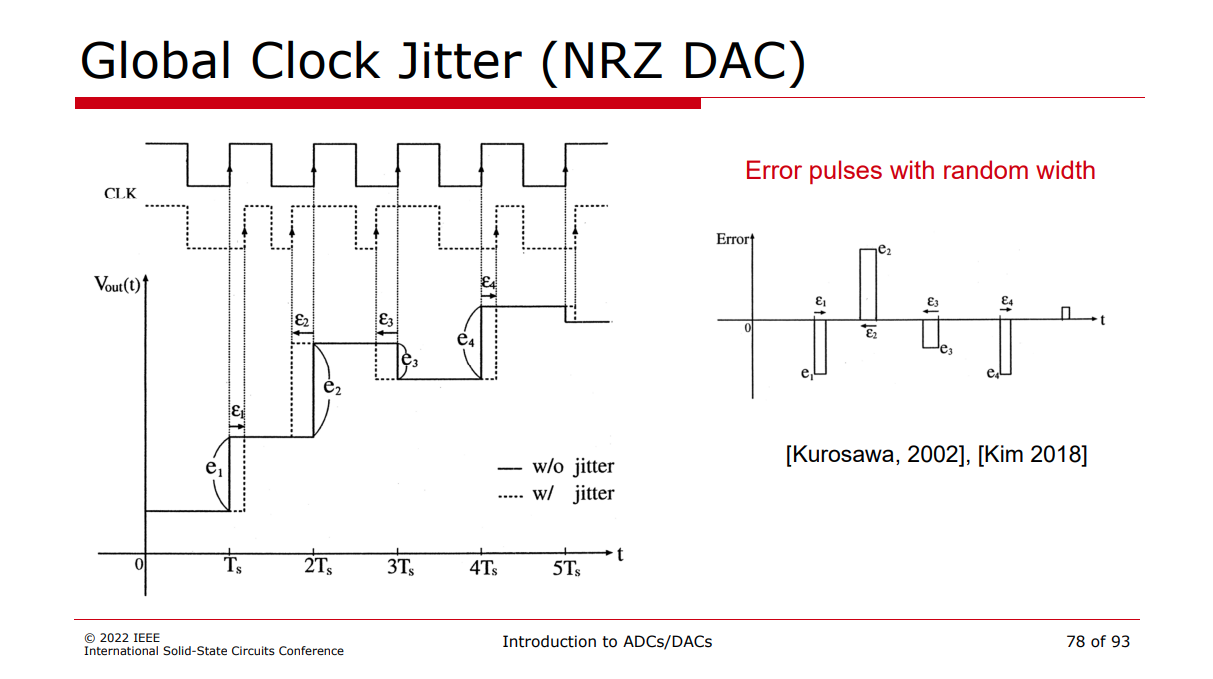
Boris Murmann ISSCC 2022 SC1: Introduction to ADCs/DACs: Metrics, Topologies, Trade Space, and Applications [pdf]
S. Kim, K. -Y. Lee and M. Lee, "Modeling Random Clock Jitter Effect of High-Speed Current-Steering NRZ and RZ DAC," in IEEE Transactions on Circuits and Systems I: Regular Papers, vol. 65, no. 9, pp. 2832-2841, Sept. 2018 [https://sci-hub.se/10.1109/TCSI.2018.2821198]
Martin Clara. High-Performance D/A-Converters - Application to Digital Transceivers, 2013 [pdf]
Chun-Hsien Su (蘇純賢). Design of Oversampled Sigma-Delta Data Converters. July, 2006 [pdf]
Cyclostationary Noise (Modulated Noise)
[https://ece-research.unm.edu/bsanthan/ece541/cyclo.pdf]
Chembian Thambidurai, "Power Spectral Density of Pulsed Noise Signals" [link]
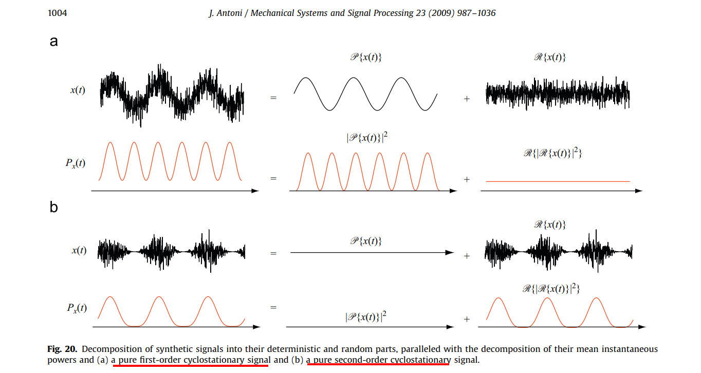
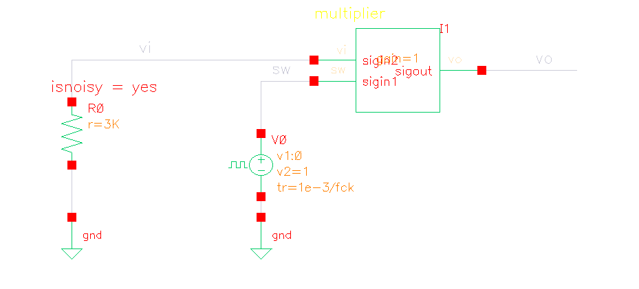
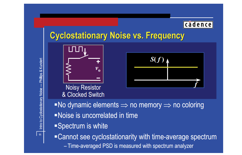
White Noise Modulation
Noisy Resistor & Clocked Switch
\[ v_t (t) = v_i(t)\cdot m_t(t) \]
where \(v_i(t)\) is input white noise, whose autocorrelation is \(A\delta(\tau)\), and \(m_t(t)\) is periodically operating switch, then autocorrelation of \(v_t(t)\) \[\begin{align} R_t (t_1, t_2) &= E[v_t(t_1)\cdot v_t(t_2)] \\ &= R_i(t_1, t_2)\cdot m_t(t_1)m_t(t_2) \end{align}\]
Then \[\begin{align} R_t(t, t-\tau) &= R_i(\tau)\cdot m_t(t)m_t(t-\tau) \\ & = A\delta(\tau) \cdot m_t(t)m_t(t-\tau) \\ & = A\delta(\tau) \cdot m_t(t) \end{align}\] Because \(m_t(t)=m_t(t+T)\), \(R_t(t, t-\tau)\) is is periodic in the variable \(t\) with period \(T\)
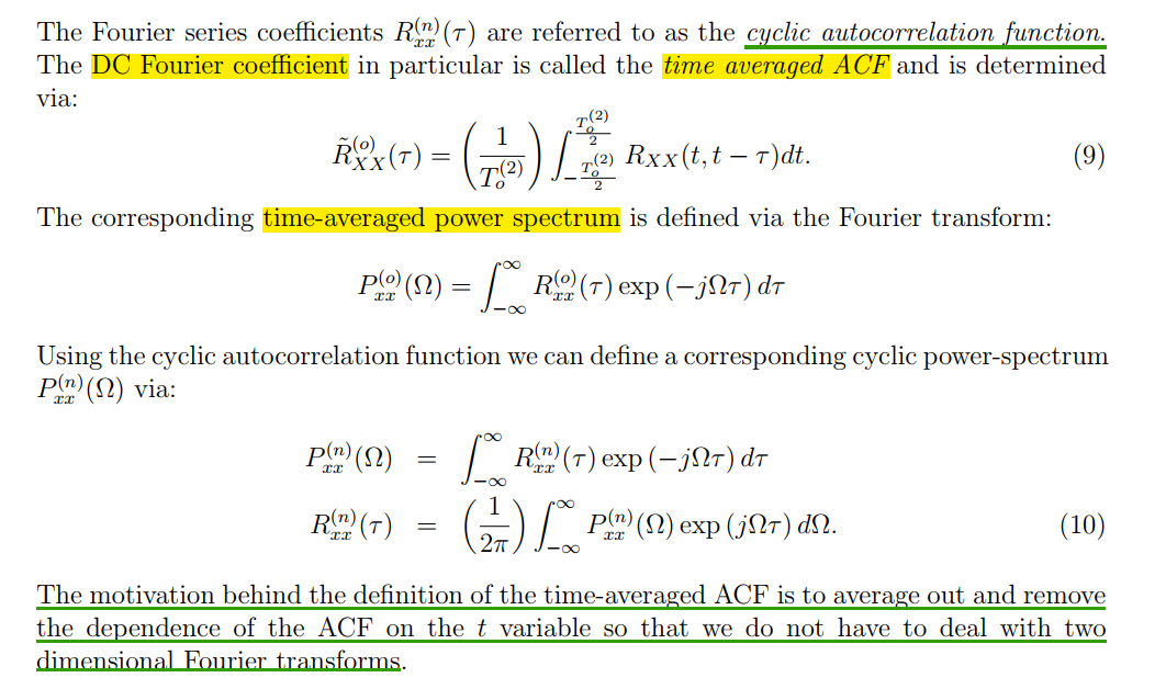
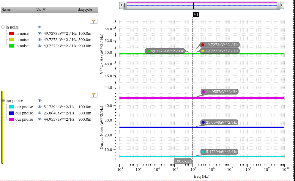
The time-averaged ACF is denoted as \(\tilde{R_t}(\tau)\)
\[ \tilde{R}_{t}(\tau) = m\cdot A\delta(\tau) \] That is, \[ S_t(f) = m\cdot S_{A}(f) \]
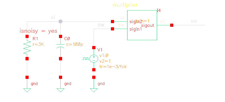
Colored Noise Modulation
 \[
\tilde{R_t}(\tau) = R_i(\tau)\cdot m_{tac}(\tau)
\]
\[
\tilde{R_t}(\tau) = R_i(\tau)\cdot m_{tac}(\tau)
\]
where \(m_t(t)m_t(t-\tau)\) averaged on \(t\) is denoted as \(m_{tac}(\tau)\) or \(\overline{m_t(t)m_t(t-\tau)}\)
The DC value of \(m_{tac}(\tau)\) can be calculated as below
for \(m\le 0.5\), the DC value of \(m_{tac}(\tau)\) \[ \frac{m\cdot mT}{T} = m^2 \]
for \(m\gt 0.5\), the DC value of \(m_{tac}(\tau)\) \[ \frac{(m+2m-1)(1-m)T + (2m-1)\{mT -(1-m)T\}}{T} = m^2 \]
Therefore, time-average power spectral density and total power are scaled by \(m^2\) in fundamental frequency sideband
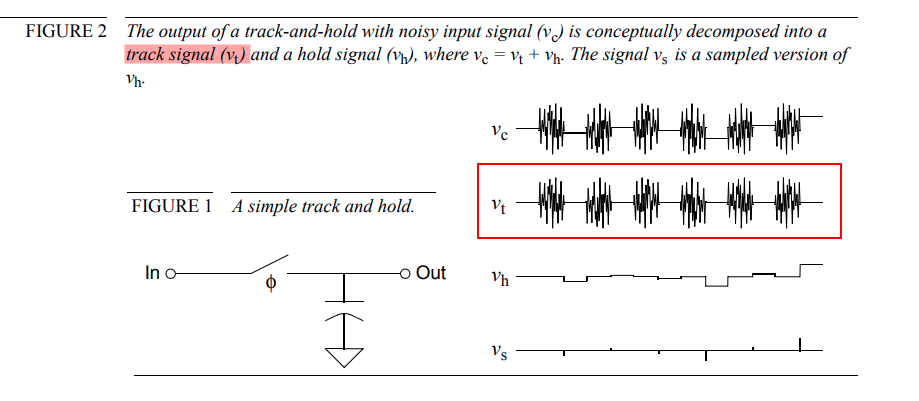
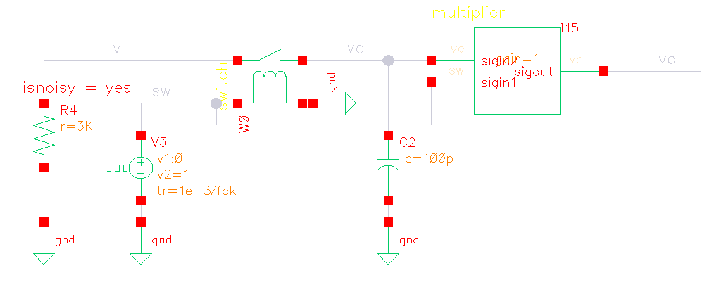
Switched-Capacitor Track signal
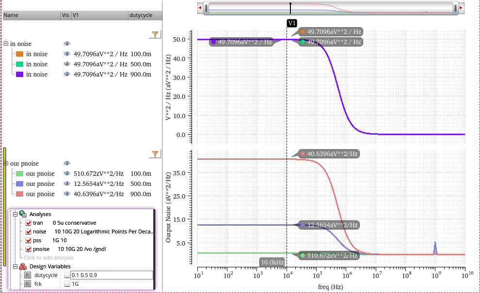
track signal pnoise (sc)
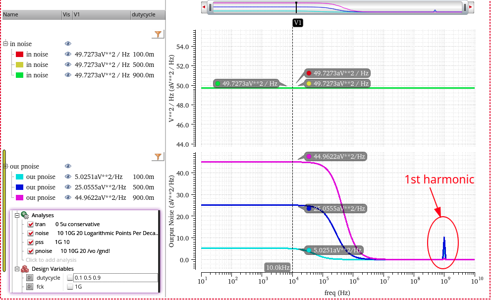
zoom in first harmonic by linear step of pnoise
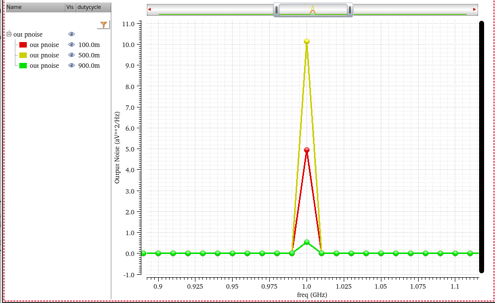
decreasing the rising/falling time of clock, the harmonics still retain
equivalent circuit for pnoise (eq)
- thermal noise of R is modulated at first
- then filtered by ideal filter
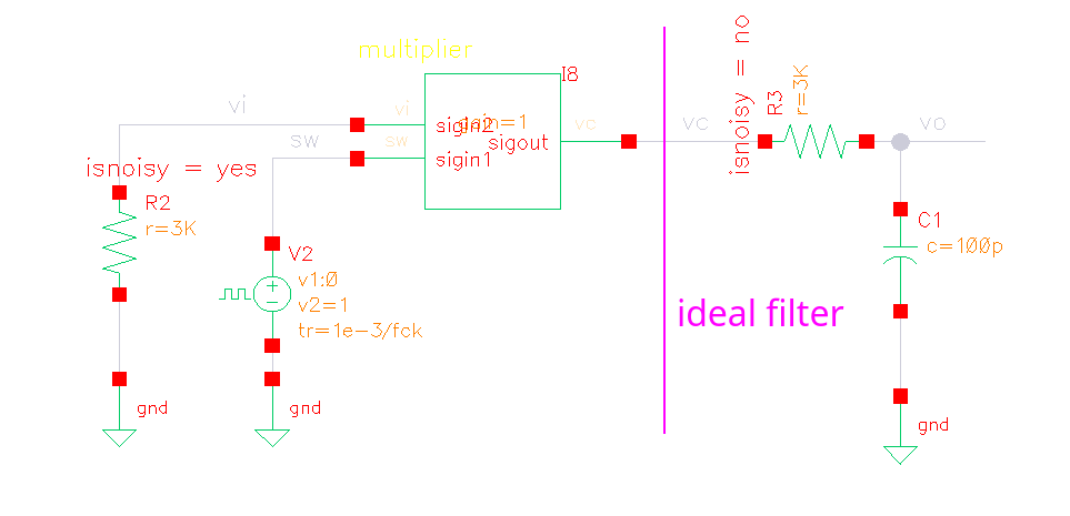
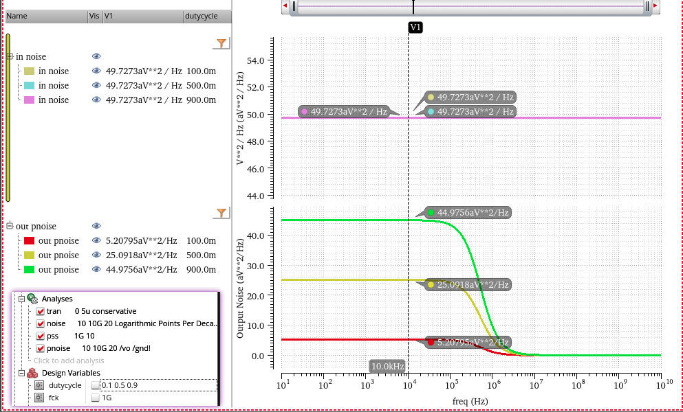
sc vs eq
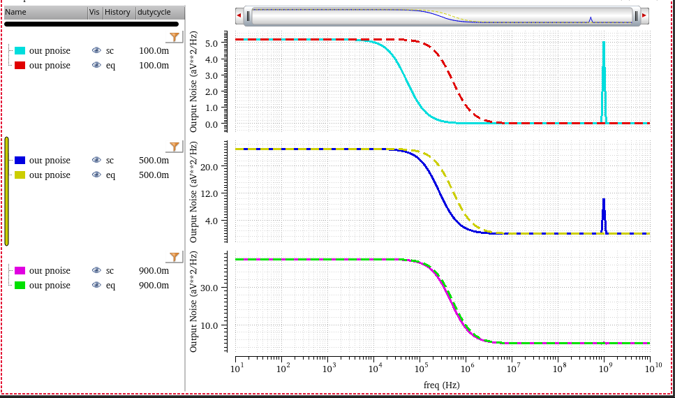
- sc: harmonic distortion
- eq: no harmonic distortion
Non-Stationary Processes (Comparator)
T. Sepke, P. Holloway, C. G. Sodini and H. -S. Lee, "Noise Analysis for Comparator-Based Circuits," in IEEE Transactions on Circuits and Systems I: Regular Papers, vol. 56, no. 3, pp. 541-553, March 2009 [https://dspace.mit.edu/bitstream/handle/1721.1/61660/Speke-2009-Noise%20Analysis%20for%20Comparator-Based%20Circuits.pdf]
Sepke, Todd. "Comparator design and analysis for comparator-based switched-capacitor circuits." (2006). [https://dspace.mit.edu/handle/1721.1/38925]
| WSS white noise input | 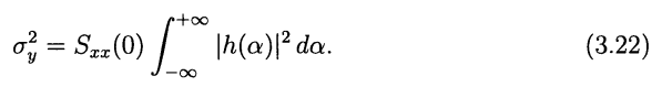 |
 |
| white noise step input | 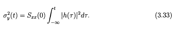 |
 |
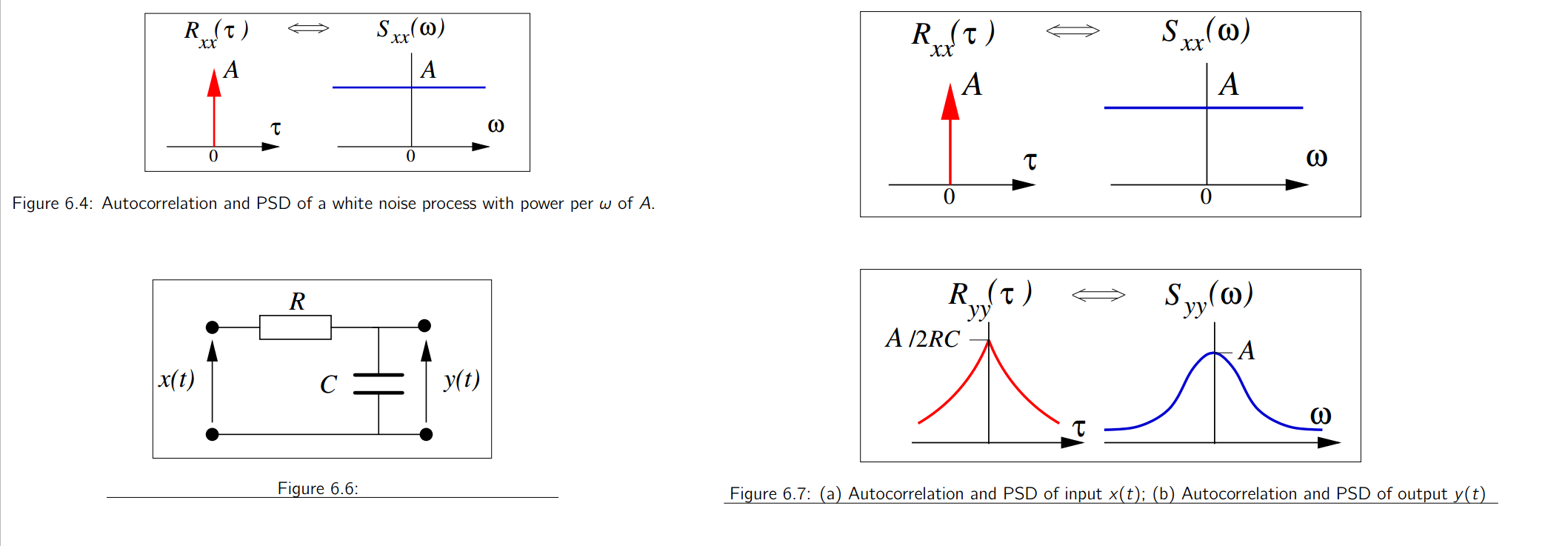
Wide-Sense-Stationary Noise
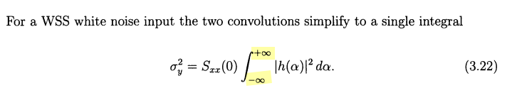
Much like sinusoidal-steady-state signal analysis, steady-state noise analysis methods assume an input \(x(t)\) of infinite duration, which is a Wide-Sense Stationary (WSS) random process
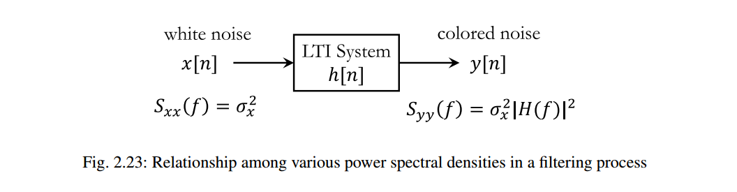
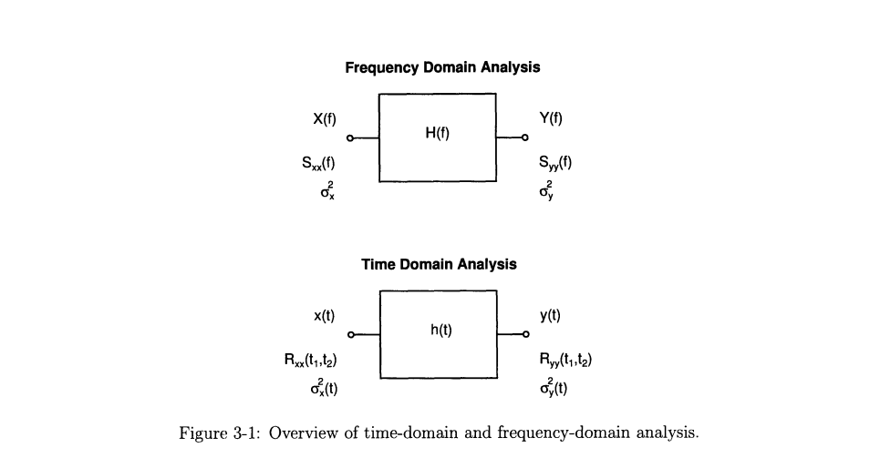
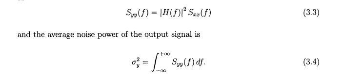
Frequency-domain Analysis
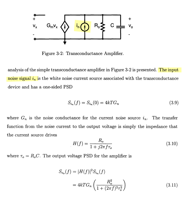
Time-domain Analysis
The output \(y(t)\) of a linear time-invariant (LTI) system \(h(t)\) \[\begin{align} R_{yy}(\tau) &= R_{xx}(\tau)*[h(\tau)*h(-\tau)] \\ &= S_{xx}(0)\delta(\tau) * [h(\tau)*h(-\tau)] \\ &= S_{xx}(0)[h(\tau)*h(-\tau)] \\ &= S_{xx}(0) \int_\alpha h(\alpha)h(\alpha-\tau)d\alpha \end{align}\]
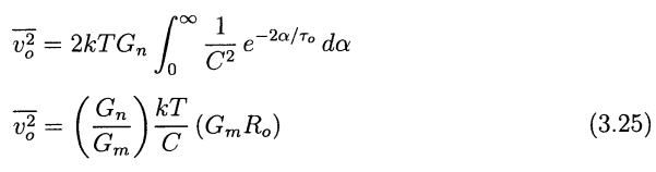
with WSS white noise input \(x(t)\), \(R_{xx}(\tau)=S_{xx}(0)\delta(\tau)\), therefore
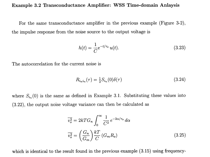
\[ V_o(s) = \frac{1}{C}\frac{RC}{1+sRC}\cdot I_n(s) \overset{\mathcal{L}} {\longrightarrow} \frac{1}{C}e^{-t/\tau_0} \]
where \(\tau_0 = RC\)
Non-stationary Noise
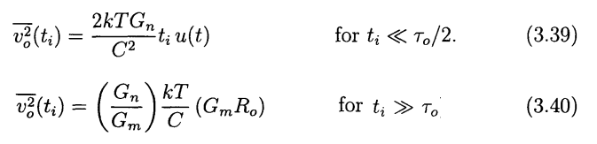
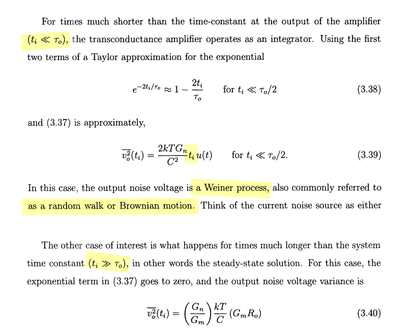
Assuming the noise applied duration is much less than the time constant, the output voltage does not reach steady-state and WSS noise analysis does not apply
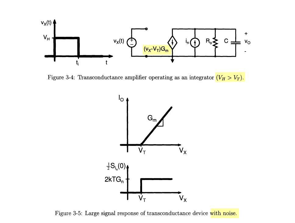
Time-domain Analysis
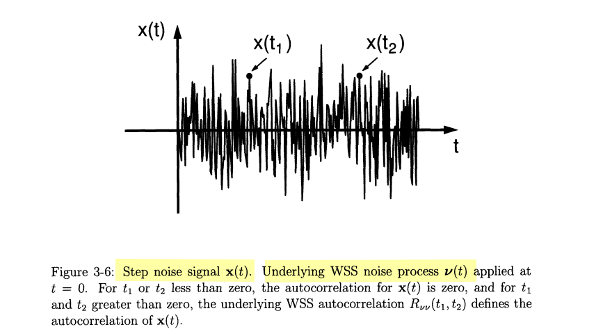
The step noise input \(x(t) = \nu(t)u(t)\) where an underlying
WSS process \(\nu(t)\) \[
R_{xx}(t_1,t_2) = E[x(t_1)x(t_2)] = R_{\nu\nu}(t_1,
t_2)u(t_1)u(t_2)=R_{\nu\nu}(t_1, t_2) \tag{3.28}
\] 
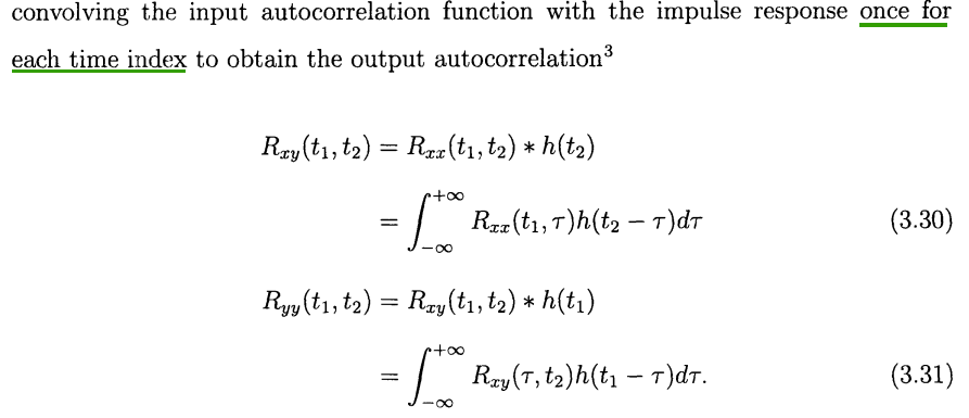
\[ R_{xy}(t_1, t_2) = E[x(t_1)y(t_2)] = E[x(t_1)(x(t_2)*h(t_2))] = E(x(t_1)x(t_2))*h(t_2) = R_{xx}(t_1,t_2)*h(t_2) \]
\[ R_{yy}(t_1,t_2) = E[y(t_1)y(t_2)] = E[(x(t_1)*h(t_1))y(t_2)] = E[x(t_1)y(t_2)]*h(t_1)=R_{xy}(t_1,t_2)*h(t_1) \]
the absolute value of each time index is important for a non-stationary signal, and only the time difference was important for WSS signals
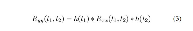
\[\begin{align} R_{yy}(t_1,t_2) &= h(t_1)*R_{\nu\nu}(t_1, t_2)*h(t_2) \\ &= h(t_1)*S_{xx}(0)\delta(t_2-t_1)*h(t_2) \\ &=S_{xx}(0) h(t_1)*(\delta(t_2-t_1)*h(t_2)) \\ &= S_{xx}(0)h(t_1)*h(t_2-t_1) \\ &= S_{xx}(0)\int_\tau h(\tau)h(t_2-t_1+\tau))d\tau \end{align}\]
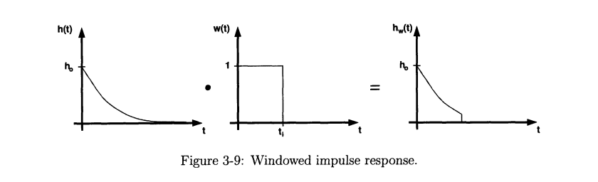
That is \[ \sigma^2_y (t)= R_{yy}(t_1,t_2)|_{t_1=t_2=t}=S_{xx}(0)\int_{-\infty}^t |h(\tau)|^2d\tau \tag{3.33} \]
\(t\), the upper limit of integration is just intuitive, which lacks strict derivation
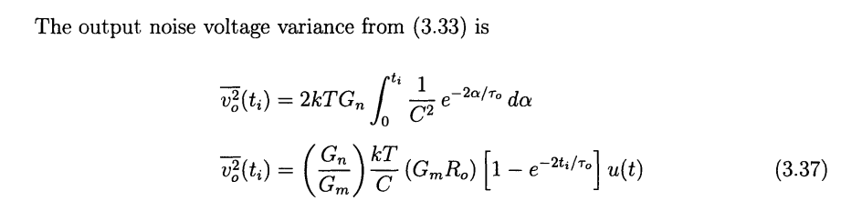
Because stable systems have impulse responses that decay to zero as time goes to infinity, the output noise variance approaches the WSS result as time approaches infinity
Richard Schreier. ECE1371 Advanced Analog Circuits Lecture 8 - COMPARATOR & FLASH ADC DESIGN [http://individual.utoronto.ca/schreier/lectures/2015/8-6.pdf]
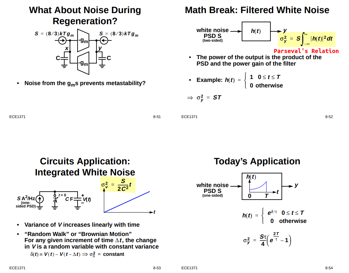
\[ R_{yy}(0) = \frac{1}{2\pi}\int_{-\infty}^{\infty}|H(\omega)|^2S_{xx}(\omega)d\omega = S \cdot \frac{1}{2\pi}\int_{-\infty}^{\infty}|H(\omega)|^2d\omega \overset{\text{Parseval's Relation}}{=} S\cdot \int_{-\infty}^{\infty}|h(t)|^2dt \]
Frequency-domain Analysis
Because the definition of the PSD assumes that the variance of the noise process is independent of time, the PSD of a non-stationary process is not very meaningful
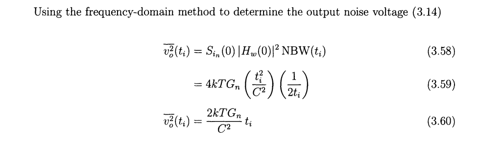
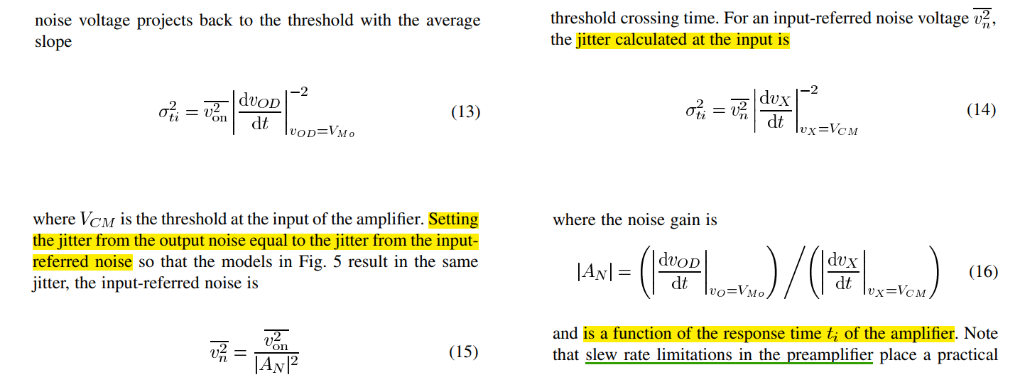
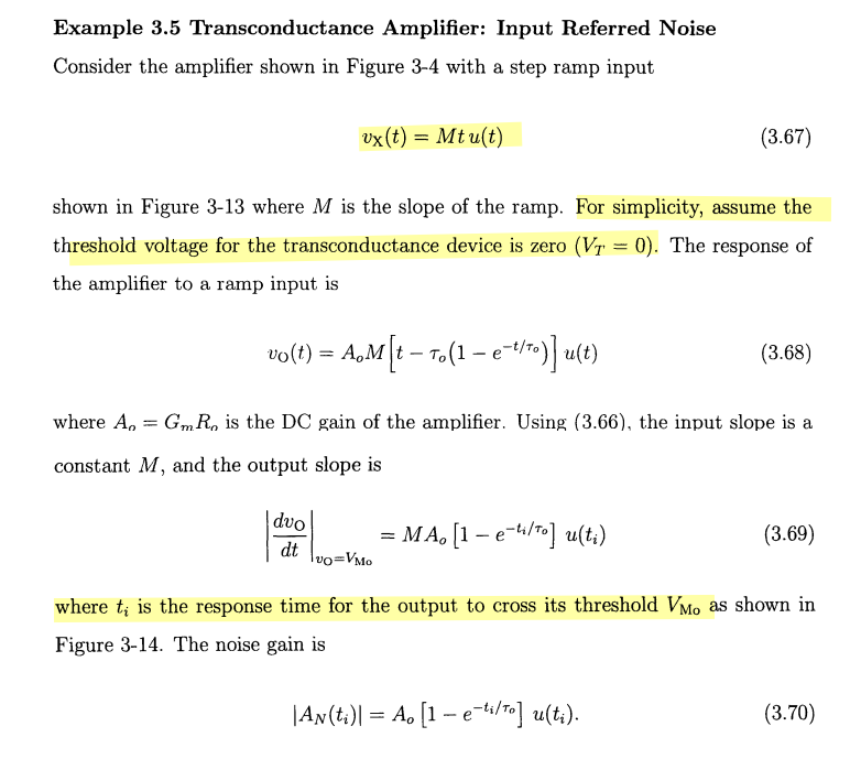
Input Referred Noise
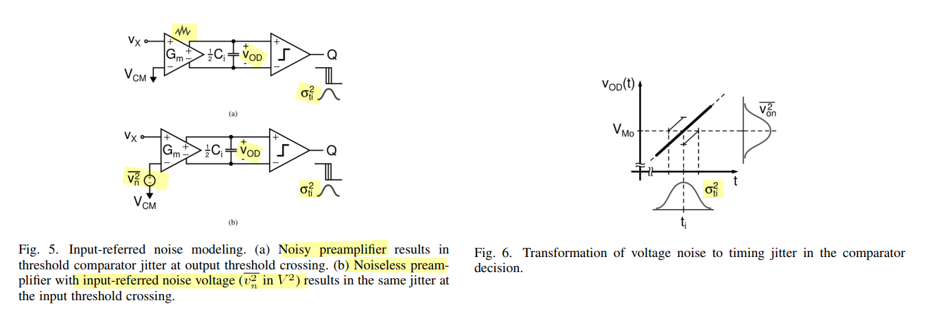
Noise Voltage to Timing Jitter Conversion & noise gain
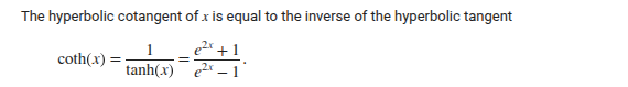
\[\begin{align} \overline{v_n^2}(t_i) &= \frac{\overline{v_{on}^2}}{|A_N|^2} \\ &= \frac{G_n}{G_m}\frac{kT}{C}\frac{1}{A_0}\frac{1+e^{-t_i/\tau_o}}{1-e^{-t_i/\tau_o}} \\ &=4kT\frac{G_n}{G_m^2}\frac{1}{4R_oC} \coth(\frac{t_i}{2\tau_o}) \\ &= 4kTR_n\frac{1}{4\tau_o} \coth(\frac{t_i}{2\tau_o}) \end{align}\]
where \(R_n = \frac{G_n}{G_m^2}\), the equivalent thermal noise resistance
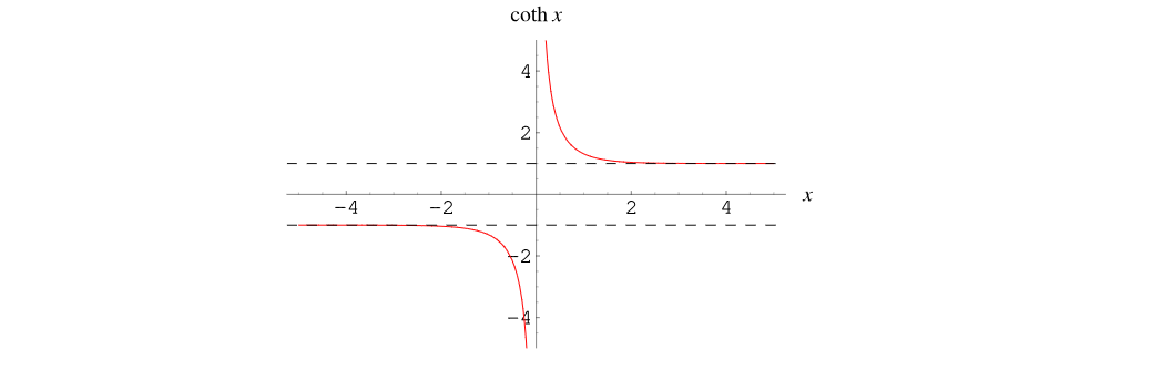
Suppose \(t_i \ll \tau_0\) \[ \overline{v_n^2}(t_i) = 4kTR_n\frac{1}{4\tau_o} \coth(\frac{t_i}{2\tau_o}) \approx 4kTR_n\frac{1}{4\tau_o} \frac{1 + (1-\frac{t_i}{\tau_0})}{1 - (1-\frac{t_i}{\tau_0})} =4kTR_n \cdot \frac{1}{2t_i} \]
Suppose \(t_i \gg \tau_0\) \[ \overline{v_n^2}(t_i) = 4kTR_n\frac{1}{4\tau_o} \coth(\frac{t_i}{2\tau_o}) \approx 4kTR_n\frac{1}{4\tau_o} = \frac{G_n}{G_m}\frac{kT}{C}\frac{1}{A_0} \] As expected, the input referred noise voltage is \(kT/C\) noise
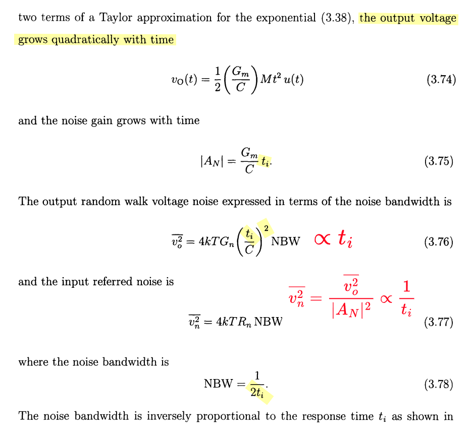
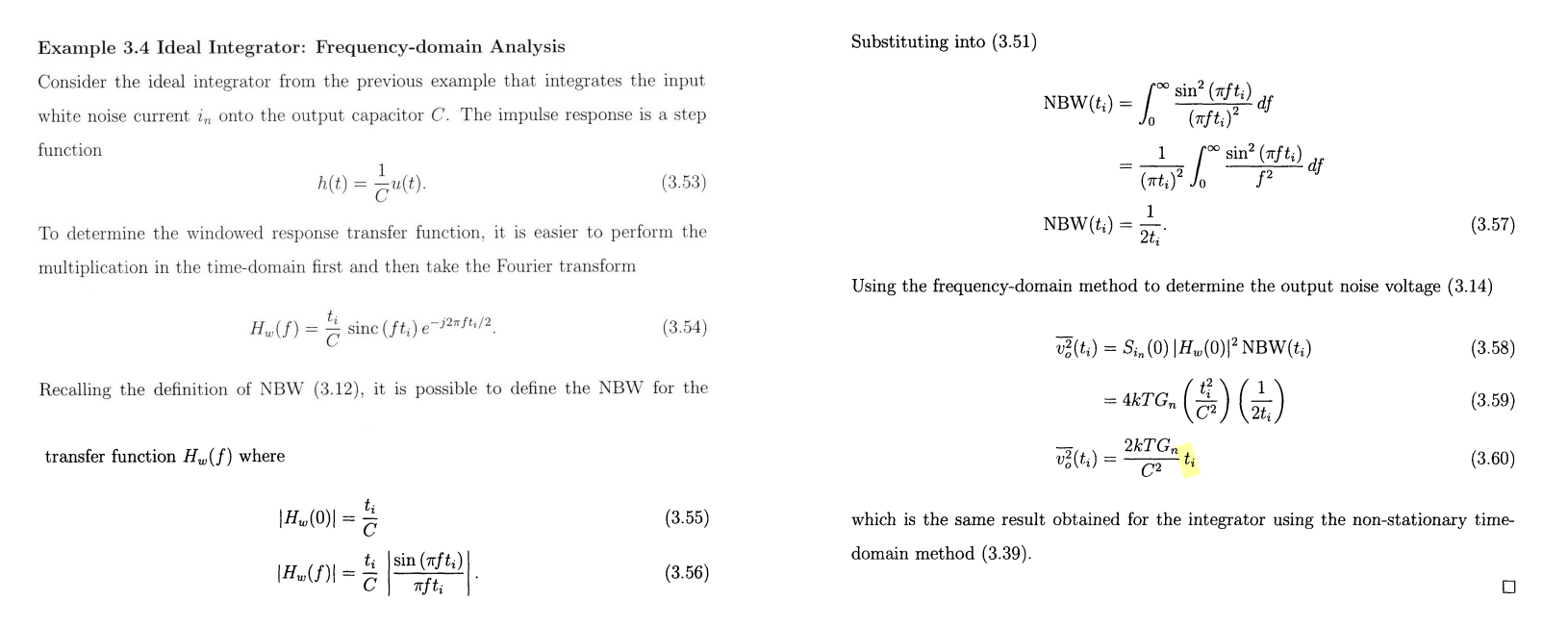
Windowed Integrals of Noise
A. A. Abidi, "Phase Noise and Jitter in CMOS Ring Oscillators," in IEEE Journal of Solid-State Circuits, vol. 41, no. 8, pp. 1803-1816, Aug. 2006 [pdf]
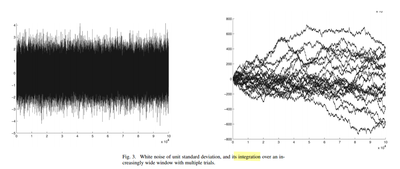
Lossless Integral
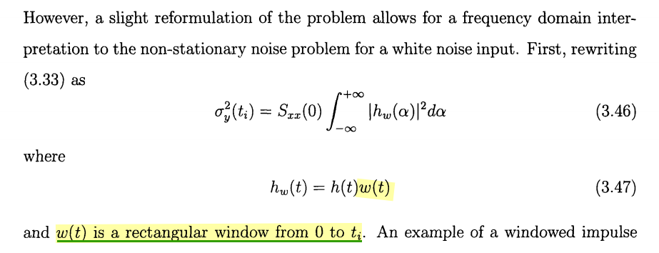
a noise current integrates onto a capacitor only
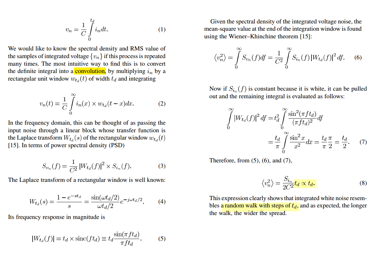
With white Gaussian noise at the input, the output spectrum is no longer white although its distribution remains Gaussian
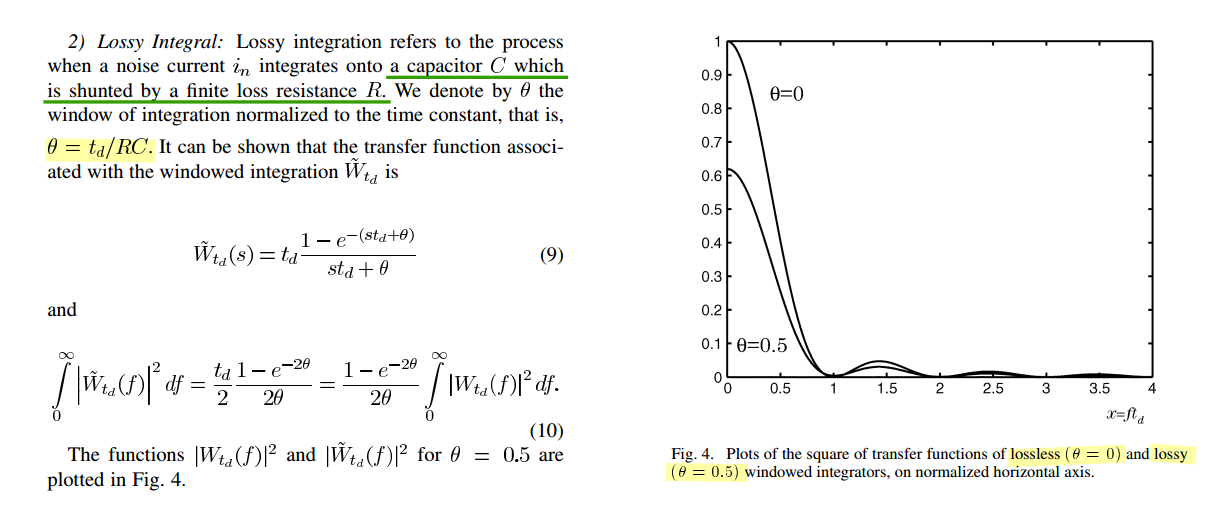
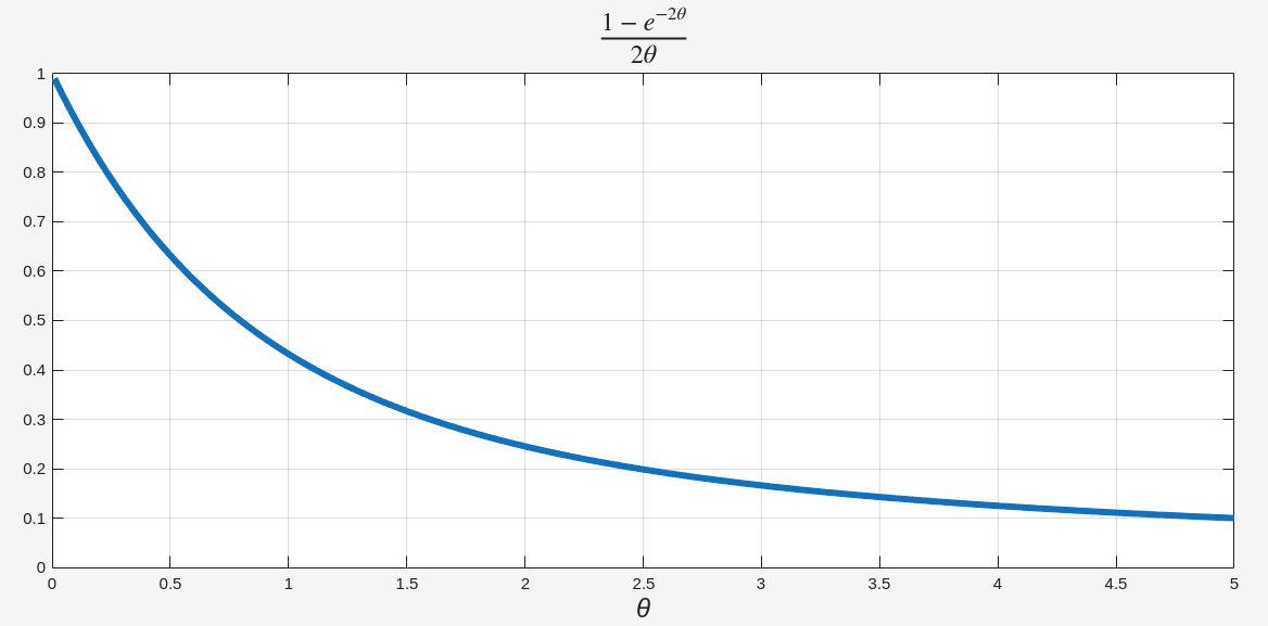
Lossy Integral
a noise current integrates onto a capacitor which is shunted by a finite loss resistance
\[ \frac{V}{I}(s) = \frac{1}{C}\frac{RC}{1+sRC} \overset{\mathcal{L}^{-1}}{\longrightarrow}\frac{1}{C}\cdot e^{-\frac{t}{RC}} \]
Laplace transform of Truncated Impulse Response \(0 \to t_d\) \[ \int_{0}^{t_d}\frac{1}{C}\cdot e^{-\frac{t}{RC}} \cdot e^{-st}dt = \frac{1}{C}\cdot \frac{1}{s+\frac{1}{RC}}\left(1-e^{-(st_d+\theta)}\right)=\frac{1}{C}\cdot \color{red}\frac{t_d}{st_d+\theta}\left(1-e^{-(st_d+\theta)}\right) \]
Google AI Mode [https://share.google/aimode/O6rjWM1YWel0NudI7]
reference
David Herres, The difference between signal under-sampling, aliasing, and folding URL: https://www.testandmeasurementtips.com/the-difference-between-signal-under-sampling-aliasing-and-folding-faq/
Pharr, Matt; Humphreys, Greg. (28 June 2010). Physically Based Rendering: From Theory to Implementation. Morgan Kaufmann. ISBN 978-0-12-375079-2. Chapter 7 (Sampling and reconstruction)
Alan V Oppenheim, Ronald W. Schafer. Discrete-Time Signal Processing, 3rd edition
Mathuranathan Viswanathan. Digital Modulations using Matlab: Build Simulation Models from Scratch