Systems, Modulation and Noise
Modulation of WSS process
Balu Santhanam, Probability Theory & Stochastic Process 2020: [Modulation of Random Processes]
Chembian Thambidurai, "Power Spectral Density of Pulsed Noise Signals" [link]

| Case | Signal | Carrier phase | Ensemble ACF | Stationarity | PSD / averaged PSD |
|---|---|---|---|---|---|
| Oscillator with small random phase noise | \(v(t)=A\sin(\omega_0t+\varphi(t))\) | fixed carrier \(\omega_0t\), small random \(\varphi(t)\) | \(\displaystyle R_v(t,\tau)\) contains terms like \(\cos(2\omega_0t+\omega_0\tau)\) | Cyclostationary, not WSS | Time-averaged: \(\displaystyle S_v(f)=\frac{A^2}{4}\left[\delta(f-f_0)+\delta(f+f_0)+S_\varphi(f-f_0)+S_\varphi(f+f_0)\right]\) |
| Random process × random-phase cosine | \(Y(t)=X(t)\cos(\Omega_c t+\Theta)\) | \(\Theta\sim U[0,2\pi)\) | \(\displaystyle R_{YY}(\tau)=\frac{R_{XX}(\tau)}{2}\cos(\Omega_c\tau)\) | WSS, if \(X(t)\) is WSS | \(\displaystyle P_{YY}(\Omega)=\frac{P_{XX}(\Omega+\Omega_c)+P_{XX}(\Omega-\Omega_c)}{4}\) |
| Random process × deterministic cosine | \(S(t)=m(t)\cos(\Omega_c t+\phi_0)\) | fixed \(\phi_0\) | \(\displaystyle R_{SS}(t,\tau)=\frac{R_{mm}(\tau)}{2}\left[\cos(\Omega_c\tau)+\cos(2\Omega_c t+\Omega_c\tau+2\phi_0)\right]\) | Cyclostationary, not WSS | Time-averaged: \(\displaystyle \tilde P_{SS}(\Omega)=\frac{P_{mm}(\Omega+\Omega_c)+P_{mm}(\Omega-\Omega_c)}{4}\) |
modulated with small perturbation
Nicola Da Dalt , Understanding Jitter and Phase Noise: 3.1.3 Voltage to Excess Phase Transformations: Random Noise
Given \(\color{blue}\phi(t)\ll 1\), the autocorrelation still depends on absolute time \(t\). Therefore \(v(t)\) is cyclostationary, and they must take a time average over one carrier period.
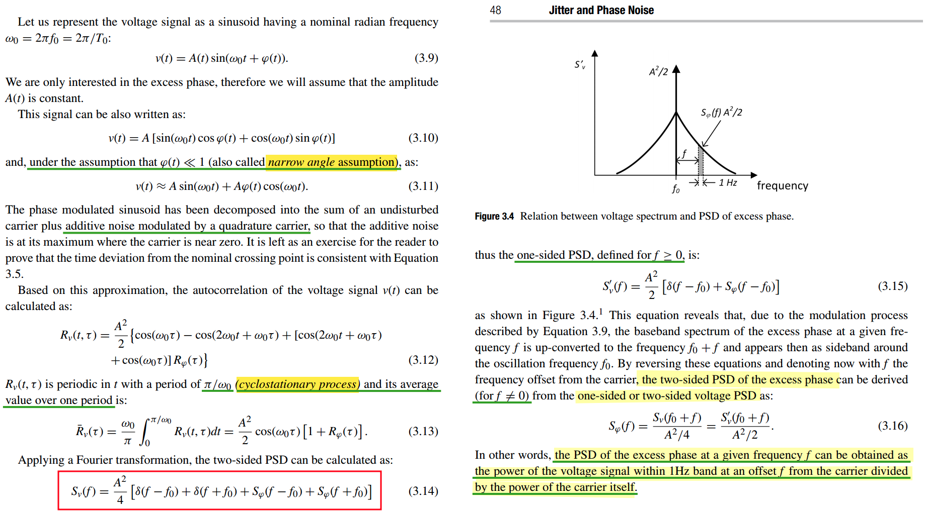
Chembiyan T. Jitter and Phase Noise in Phase Locked Loops [link]
\[ y(t) = A\cos(2\pi f_0t+\phi_n(t)) \approx A \cos(2\pi f_0 t) - A \phi_n (t)\sin(2\pi f_0 t) \]
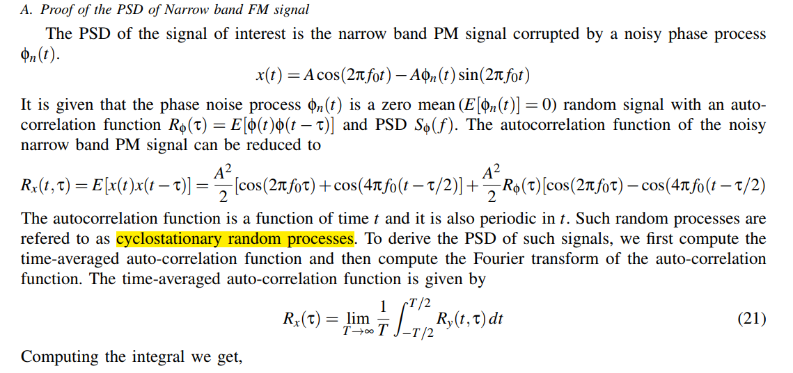 \[
R_x(\tau) = \frac{A^2}{2}\cos(2\pi f_0\tau)
+ \frac{A^2}{2}R_\phi(\tau)\cos(2\pi f_0\tau)
\] The PSD of the signal \(x(t)\) is given by \[
S_x(f) = \mathcal{F}\{R_x(\tau)\} =
\frac{P_c}{2}\left[\delta(f+f_0)+\delta(f-f_0)+S_\phi(f+f_0)+S_\phi(f-f_0)\right]
\] where \(P_c = A^2/2\) is the
carrier power of the signal
\[
R_x(\tau) = \frac{A^2}{2}\cos(2\pi f_0\tau)
+ \frac{A^2}{2}R_\phi(\tau)\cos(2\pi f_0\tau)
\] The PSD of the signal \(x(t)\) is given by \[
S_x(f) = \mathcal{F}\{R_x(\tau)\} =
\frac{P_c}{2}\left[\delta(f+f_0)+\delta(f-f_0)+S_\phi(f+f_0)+S_\phi(f-f_0)\right]
\] where \(P_c = A^2/2\) is the
carrier power of the signal
modulated with full-cycle random
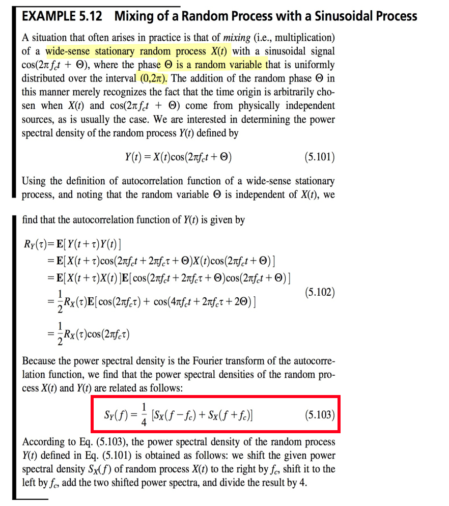
Given \(\color{blue}\Theta\sim U[0,2\pi]\), after ensemble averaging, the autocorrelation becomes WSS
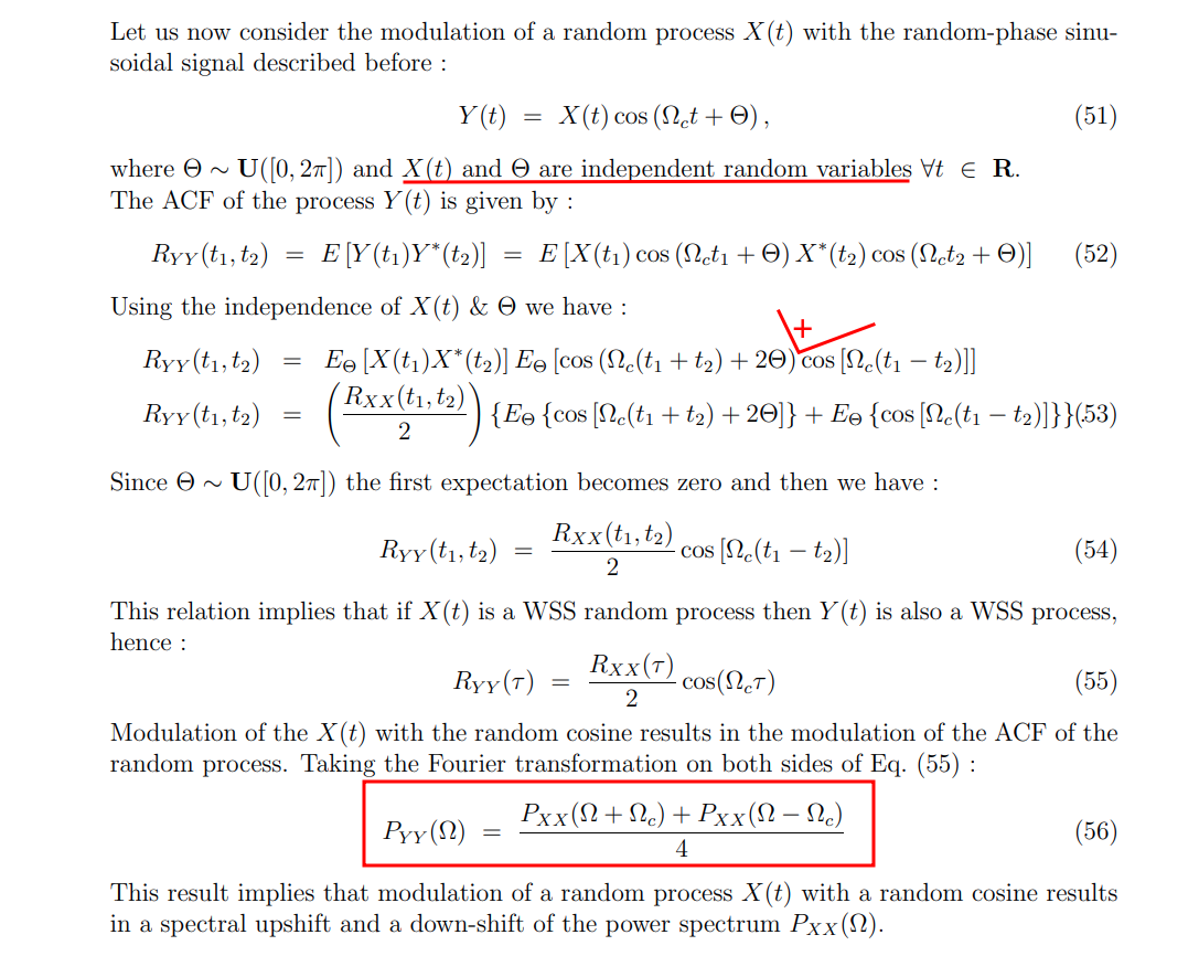
Haykin, Simon S., and Michael Moher. Communication Systems. 5th ed. John Wiley & Sons, 2009. - Mixing of a Random Process with a Sinusoidal Process
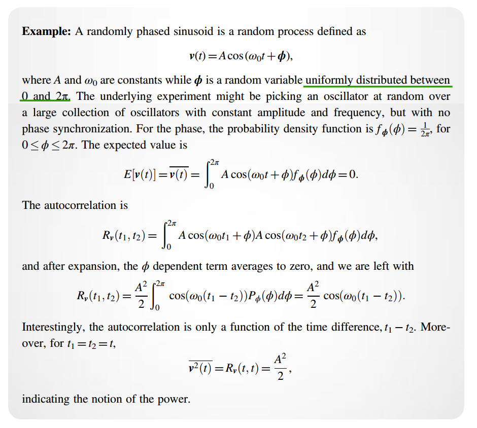
Assume \(\Theta\sim \mathcal U[0,2\pi)\) is a single random phase that remains constant for all \(t\): \[ \color{blue}\boxed{X(t)=A\cos(\omega_0t+\Theta).} \]
Mean \[ \begin{aligned} m_X(t) &=\mathbb E[X(t)]\\ &=\frac{A}{2\pi}\int_0^{2\pi} \cos(\omega_0t+\theta)\,d\theta\\ &=0. \end{aligned} \]
Thus, the mean is independent of \(t\).
Autocorrelation
For \(t_1\) and \(t_2\), \[ R_X(t_1,t_2) = \mathbb E[X(t_1)X(t_2)]. \] Using \(\cos a\cos b=\frac{1}{2}\left[\cos(a-b)+\cos(a+b)\right],\)
we obtain \[ \begin{aligned} R_X(t_1,t_2) &= \frac{A^2}{2} \mathbb E\left[ \cos\big(\omega_0(t_1-t_2)\big) + \cos\big(\omega_0(t_1+t_2)+2\Theta\big) \right]. \end{aligned} \] Since \(\Theta\) is uniform, \[ \mathbb E\left[ \cos\big(\omega_0(t_1+t_2)+2\Theta\big) \right]=0. \] Therefore, \[ \boxed{ R_X(t_1,t_2) = \frac{A^2}{2} \cos\big(\omega_0(t_1-t_2)\big) } \] or, defining \(\tau=t_1-t_2\), \[ \boxed{ R_X(\tau)=\frac{A^2}{2}\cos(\omega_0\tau) }. \] The autocorrelation depends only on the time difference \(\tau\).
Is it WSS?
Yes. The two WSS conditions are satisfied: \[ m_X(t)=0, \] which is constant, and \[ R_X(t_1,t_2)=R_X(t_1-t_2). \] Thus, \[ \boxed{X(t)\text{ is wide-sense stationary.}} \] In fact, because a time shift simply changes the uniformly distributed phase, \[ X(t+t_0) = A\cos\left(\omega_0t+\underbrace{\Theta+\omega_0t_0}_{\text{still uniform modulo }2\pi}\right), \] the process is also strict-sense stationary.
Power spectral density
Using the angular-frequency Fourier-transform convention \[ S_X(\omega) = \int_{-\infty}^{\infty} R_X(\tau)e^{-j\omega\tau}\,d\tau, \] and \[ \mathcal F\{\cos(\omega_0\tau)\} = \pi\left[ \delta(\omega-\omega_0)+\delta(\omega+\omega_0) \right], \] we get \[ \boxed{ S_X(\omega) = \frac{\pi A^2}{2} \left[ \delta(\omega-\omega_0) + \delta(\omega+\omega_0) \right] }. \] Thus, the PSD consists of two spectral lines at \(\omega=\pm\omega_0\).
The total average power is \[ R_X(0)=\frac{A^2}{2}, \] and equivalently, \[ \frac{1}{2\pi}\int_{-\infty}^{\infty}S_X(\omega)\,d\omega = \frac{A^2}{2}. \] For frequency \(f\), where \(f_0=\omega_0/(2\pi)\), \[ \color{blue}\boxed{ S_X(f) = \frac{A^2}{4} \left[ \delta(f-f_0)+\delta(f+f_0) \right] }. \] The random phase makes the ensemble stationary; a sinusoid with a fixed deterministic phase is not normally regarded as a stationary random process because it contains no random ensemble.
modulated with deterministic cosine
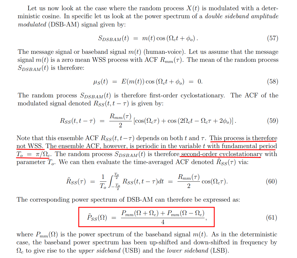
the carrier phase/time origin is fixed, not randomized, it not WSS but cyclostationary
Hayder Radha, ECE 458 Communications Systems Laboratory Spring 2008: Lecture 7 - EE 179: Introduction to Communications - Winter 2006–2007 Energy and Power Spectral Density and Autocorrelation

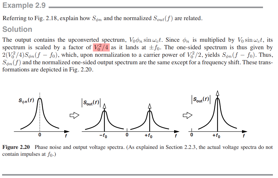
\(g(t) = i_n(t)\sin\omega_0 t\) is not WSS (it's cyclostationary), but its time-averaged PSD is white
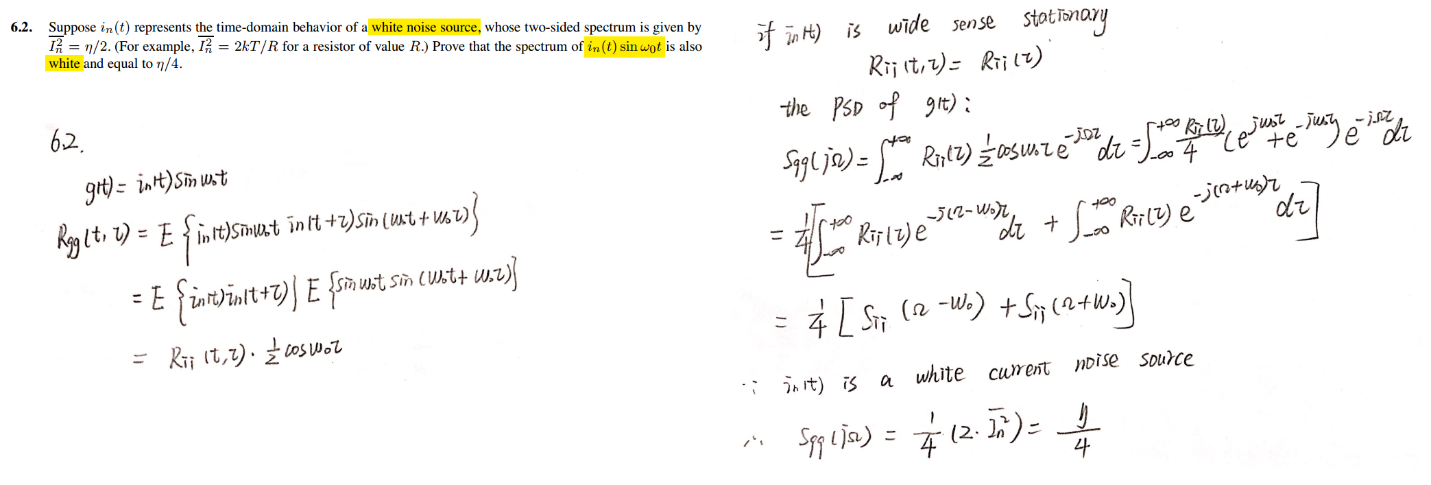
the solution silently performs the time-averaging step
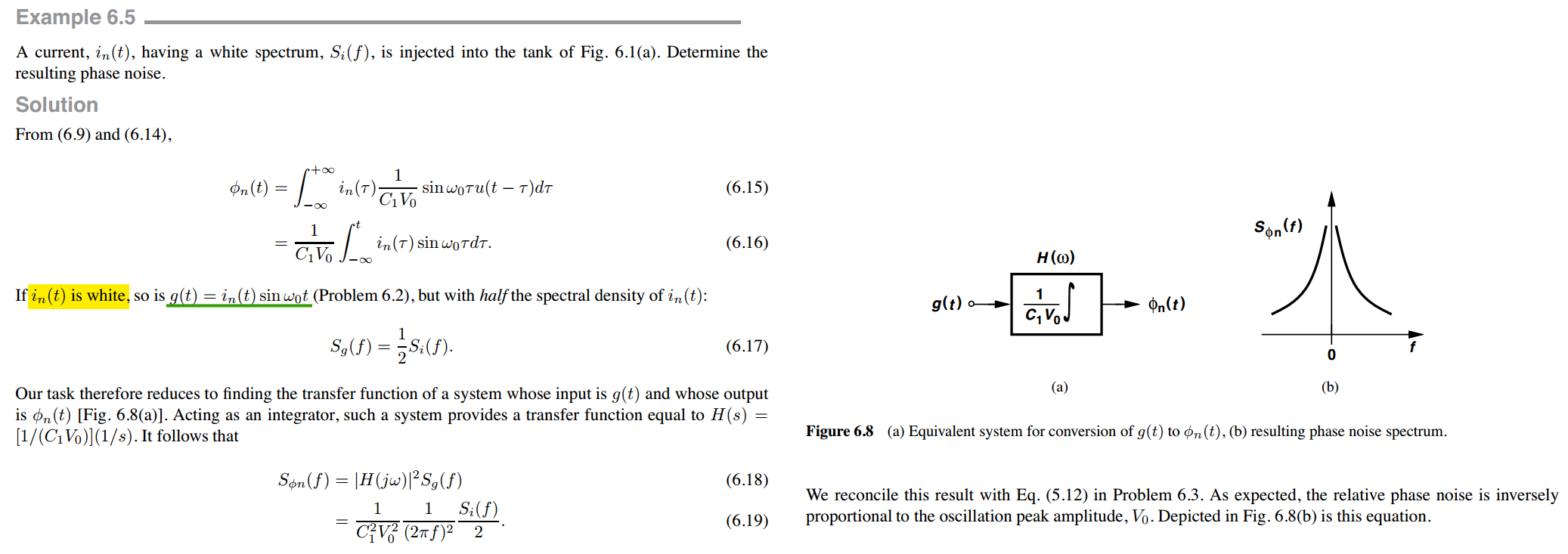
Assume zero-mean white noise \(n(t)\) is multiplied by a sinusoid:
\[ y(t)=n(t)\cos(\omega_0 t) \]
Let the two-sided white-noise PSD be
\[ S_n(f)=\frac{N_0}{2} \]
so
\[ R_n(\tau)=\frac{N_0}{2}\delta(\tau) \]
Because the sinusoid is deterministic and time-varying, \(y(t)\) is generally cyclostationary, not WSS.
Using the symmetric autocorrelation definition,
\[ R_y(t,\tau) = E\left[ y\left(t+\frac{\tau}{2}\right) y\left(t-\frac{\tau}{2}\right) \right] \]
we get
\[\begin{aligned} R_y(t,\tau) &= R_n(\tau) \cos\left(\omega_0 t+\frac{\omega_0\tau}{2}\right) \cos\left(\omega_0 t-\frac{\omega_0\tau}{2}\right) \\ &= \frac{R_n(\tau)}{2} \left[ \cos(\omega_0\tau)+\cos(2\omega_0t) \right] \end{aligned}\]
Therefore, for white noise,
\[ \boxed{ R_y(t,\tau) = \frac{N_0}{4} \left[ \cos(\omega_0\tau)+\cos(2\omega_0t) \right]\delta(\tau) } \]
If you average over one modulation period, then
\[ \overline{R_y}(\tau) = \frac12 R_n(\tau)\cos(\omega_0\tau) \]
For general stationary noise this corresponds to
\[ \boxed{ \overline{S_y}(f) = \frac14 \left[ S_n(f-f_0)+S_n(f+f_0) \right] } \]
where \(f_0=\frac{\omega_0}{2\pi}\)
For ideal white noise,
\[ S_n(f-f_0)=S_n(f+f_0)=\frac{N_0}{2} \]
so
\[ \boxed{ \overline{S_y}(f)=\frac{N_0}{4} } \]
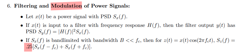
Thus an important result is: multiplying ideal white noise by a sinusoid does not change the shape of its time-averaged PSD—it remains white—but its average PSD is reduced by a factor of 2, because
\[ \overline{\cos^2(\omega_0t)}=\frac12 \]
For colored noise, however, the sinusoidal multiplication creates two shifted copies:
\[ S_n(f) \rightarrow \frac14S_n(f-f_0)+\frac14S_n(f+f_0) \]
Quadrature-Modulated Processes
Haykin, Simon S., and Michael Moher. Communication Systems. 5th ed. John Wiley & Sons, 2009.
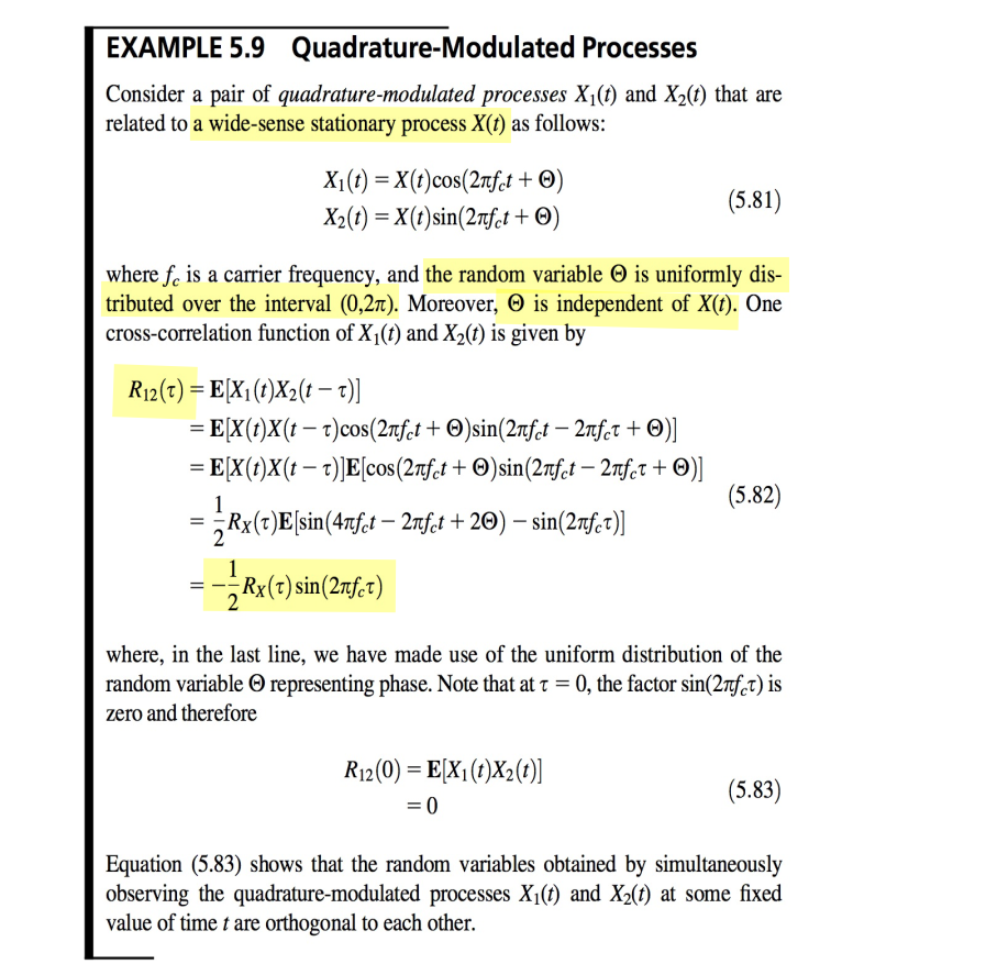
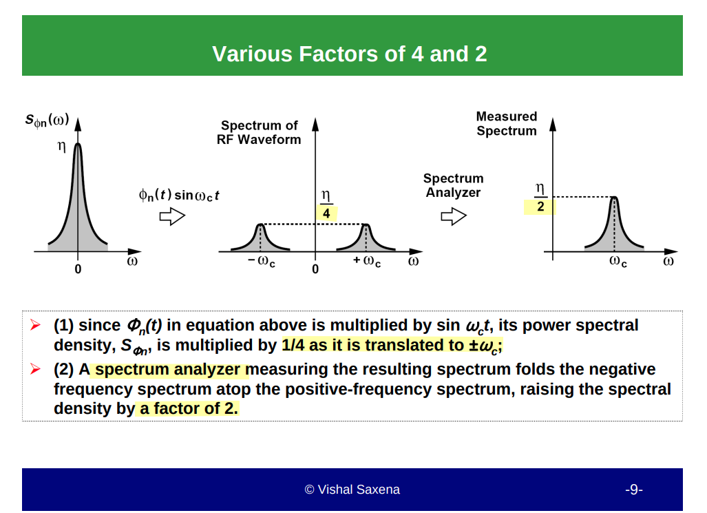
Dr. Vishal Saxena, ECE518 Memory/Clock Synchronization IC Design: Oscillator Phase Noise [https://www.eecis.udel.edu/~vsaxena/courses/ece504/Handouts/Oscillator%20Phase%20Noise.pdf]
Sampling of WSS process
Balu Santhanam, Probability Theory & Stochastic Process 2020: Impulse sampling of Random Processes
DT sequence \(x[n]\)
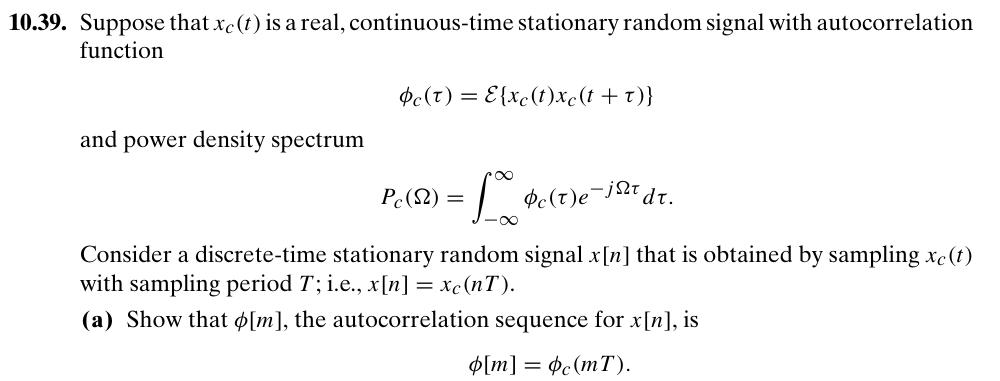
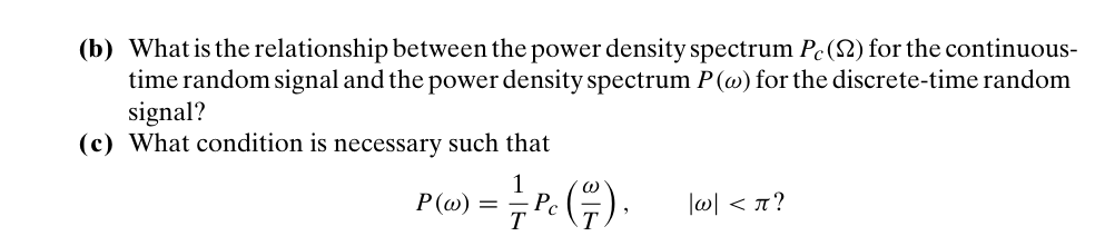
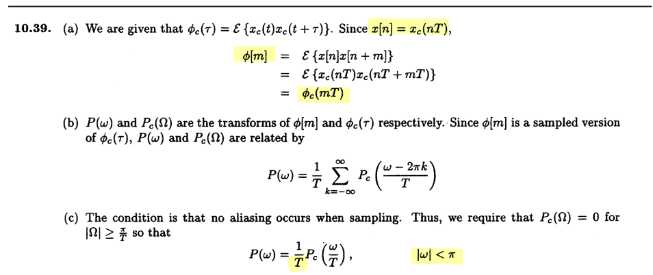
Owing to \(\phi[0] = \phi_c(0)\), the average power of the sampled version \(x[n]\) is the same as its input \(x_c(t)\)
impulse train \(x_s(t)\)
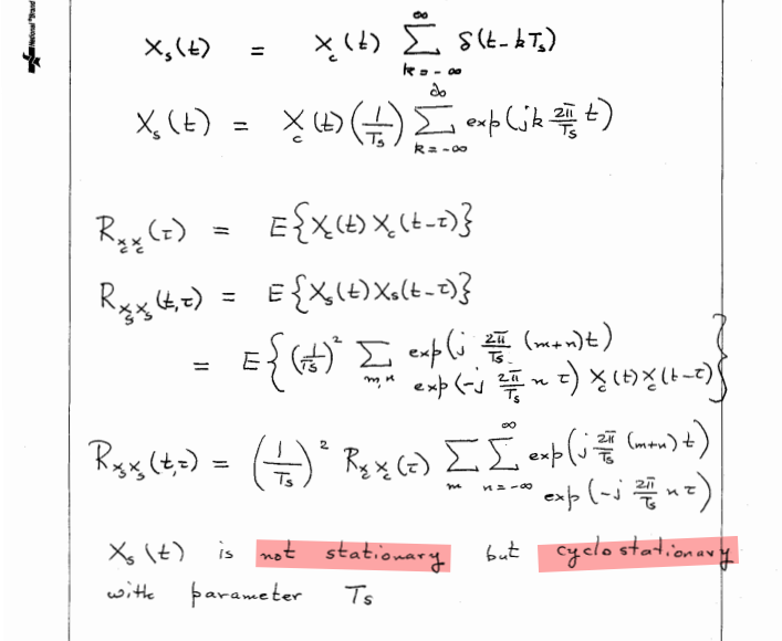
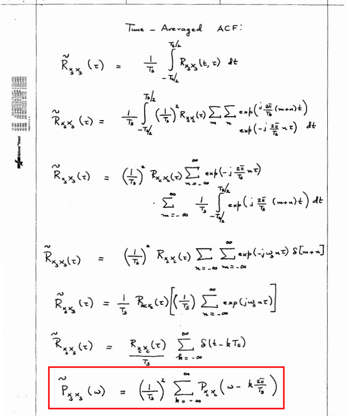
That is \[ P_{x_s x_s} (f)= \frac{1}{T_s^2}P_{xx}(f) \] where \(x[n]\) is sampled discrete-time sequence, \(x_s(t)\) is sampled impulse train
Noise Aliasing
apply foregoing observation
Pulsed Noise Signals
Chembian Thambidurai, "Power Spectral Density of Pulsed Noise Signals" [link]
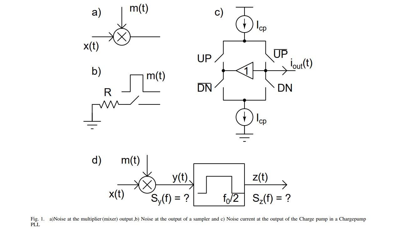
Above, the output of the multiplier be \(y(t)\) is passed through a ideal brick wall low pass filter with a bandwidth of \(f_0/2\)
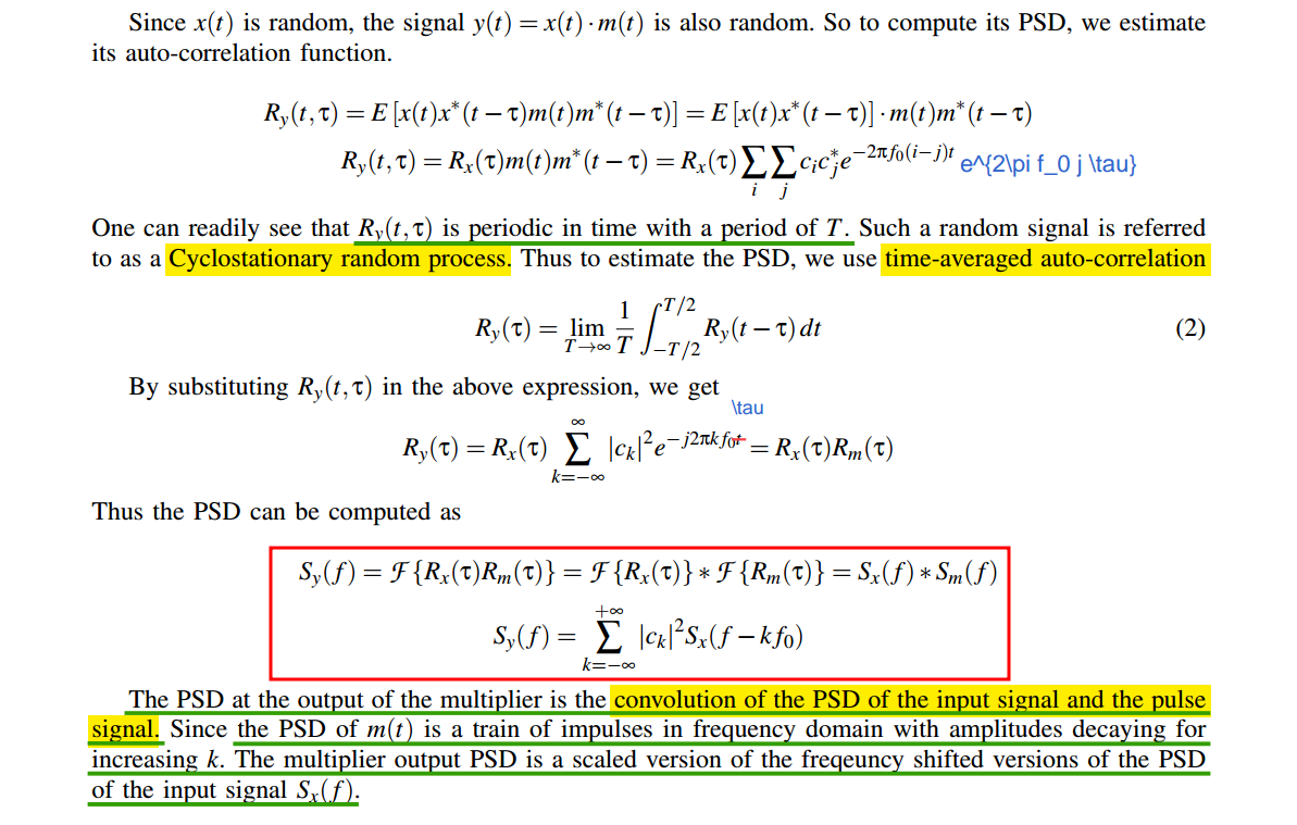
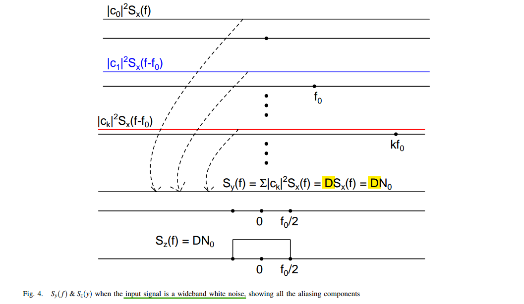
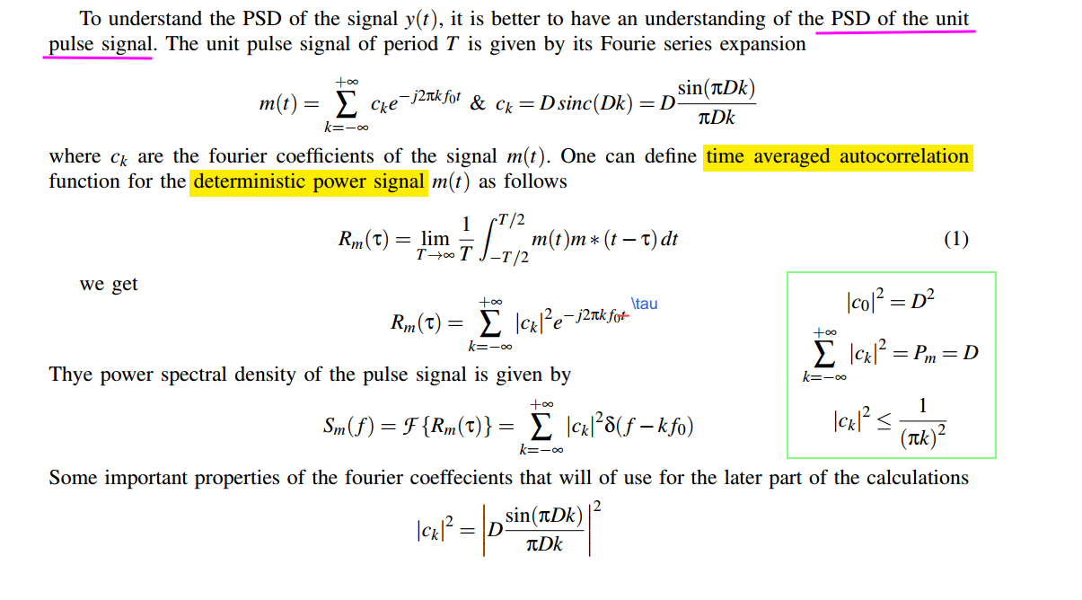
When a random signal is multiplied by a pulse function, the resulting signal becomes a cyclo-stationary random process.
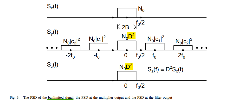
As rule of thumb, the spectrum of such a pulsed noise signal
thermal noise is multiplied by \(\color{red}D\)
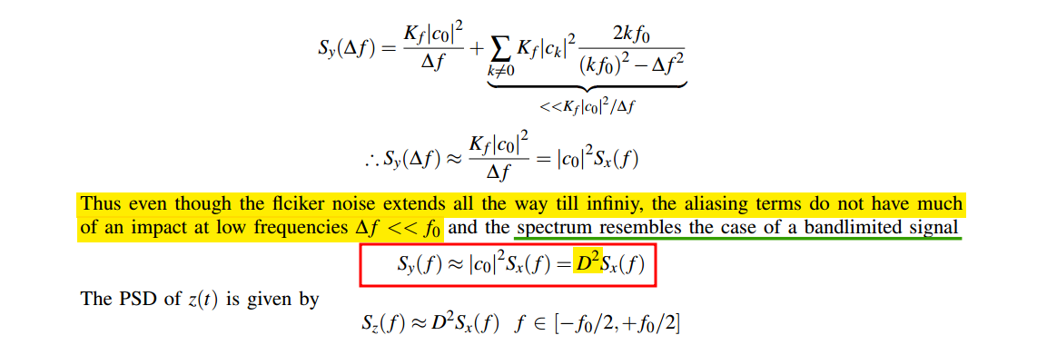
flicker noise is multiplied by \(\color{red}D^2\),
where \(D\) is the duty cycle of the pulse signal
banlimited input (no aliasing)
wideband white noise input
flicker noise input
with \(S_x(f)=\frac{K_f}{f}\)
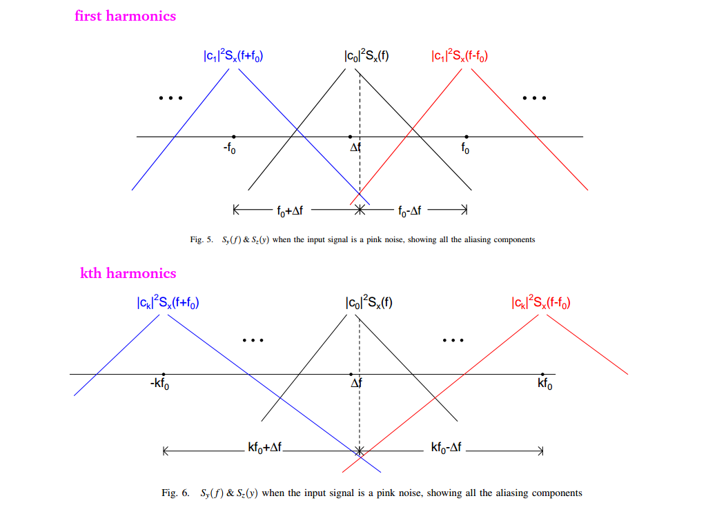

Assuming \(\Delta f \ll f_0\)
Rectangular Pulse Sampling
Balu Santhanam. ece439 Introduction to Digital Signal Processing. Example: Rectangular Pulse Sampling [http://ece-research.unm.edu/bsanthan/ece439/recsamp.pdf]
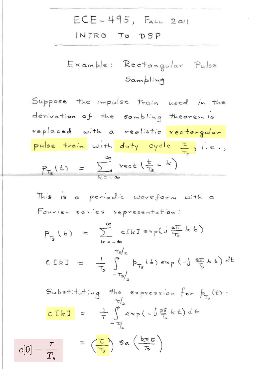
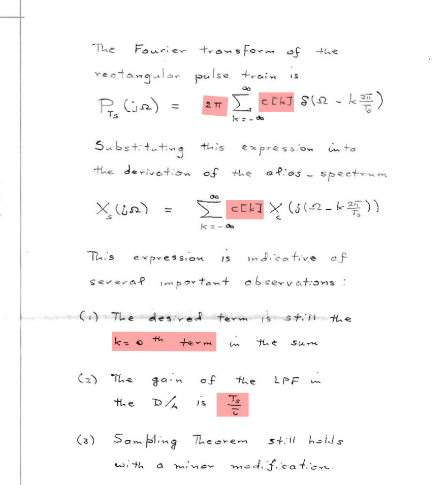
reference
Alan V Oppenheim, Ronald W. Schafer. Discrete-Time Signal Processing, 3rd edition [pdf]
R. E. Ziemer and W. H. Tranter, Principles of Communications, 7th ed., Wiley, 2013 [pdf]
John G. Proakis and Masoud Salehi, Fundamentals of communication systems 2nd ed [pdf]
Rhee, W. and Yu, Z., 2024. Phase-Locked Loops: System Perspectives and Circuit Design Aspects. John Wiley & Sons
Lacaita, Andrea Leonardo, Salvatore Levantino, and Carlo Samori. Integrated frequency synthesizers for wireless systems. Cambridge University Press, 2007
Phillips, Joel R. and Kenneth S. Kundert. "Noise in mixers, oscillators, samplers, and logic: an introduction to cyclostationary noise." Proceedings of the IEEE 2000 Custom Integrated Circuits Conference. [pdf, slides]
Antoni, J., "Cyclostationarity by examples", Mechanical Systems and Signal Processing, vol. 23, no. 4, pp. 987–1036, 2009 [https://docente.unife.it/docenti/dleglc/a-a-2010-2011-dmsm/ciclostazionarieta.pdf]
Kundert, Ken. (2006). Simulating Switched-Capacitor Filters with SpectreRF. URL:https://designers-guide.org/analysis/sc-filters.pdf
STEADY-STATE AND CYCLO-STATIONARY RTS NOISE IN MOSFETS [https://ris.utwente.nl/ws/portalfiles/portal/6038220/thesis-Kolhatkar.pdf]
Christian-Charles Enz. "High precision CMOS micropower amplifiers" [pdf]
L.W. Couch, Digital and Analog Communication Systems, 8th Edition, Pearson, 2013. [pdf]