Systems, Modulation and Noise

Posted on 2024-10-07 Edited on 2024-11-23 In dsp

asymmetric sideband

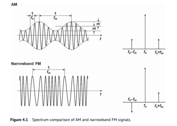
The spectrum of the narrowband FM signal is very similar to that of an amplitude modulation (AM) signal but has the phase reversal for the other sideband component

Assume the modulation frequency of PM and AM are same, \(\omega_m\)

\[\begin{align} x(t) &= (1+A_m\cos{\omega_m t})\cos(\omega_0 t + P_m \sin\omega_m t) \\ &= \cos(\omega_0 t + P_m \sin\omega_m t) + A_m\cos{\omega_m t}\cos(\omega_0 t + P_m \sin\omega_m t) \\ &= X_{pm}(t) + X_{apm}(t) \end{align}\]

\(X_{pm}(t)\), PM only part \[ X_{pm}(t) = \cos\omega_0 t - \frac{P_m}{2}\cos(\omega_0 - \omega_m)t + \frac{P_m}{2}\cos(\omega_0 + \omega_m)t \] \(X_{apm}(t)\), AM & PM part \[\begin{align} X_{apm}(t) &= A_m \cos{\omega_m t} (\cos\omega_0 t-P_m\sin\omega_m t\sin\omega_0 t) \\ &= \frac{A_m}{2}[\cos(\omega_0 + \omega_m)t + \cos(\omega_0 -\omega_m)t] - \frac{A_mP_m}{2}\sin(2\omega_m t)\sin(\omega_0 t) \\ &= \frac{A_m}{2}\cos(\omega_0 + \omega_m)t + \frac{A_m}{2}\cos(\omega_0 -\omega_m)t - \frac{A_mP_m}{4}\cos(\omega_0 - 2\omega_m)t + \frac{A_mP_m}{4}\cos(\omega_0 + 2\omega_m)t \end{align}\]

That is \[\begin{align} x(t) &= \cos\omega_0 t + \frac{A_m-P_m}{2}\cos(\omega_0 - \omega_m)t + \frac{A_m+P_m}{2}\cos(\omega_0 + \omega_m)t \\ &\space\space\space\space\space\space\space\space\space\space\space\space\space\space\space\space\space\space - \frac{A_mP_m}{4}\cos(\omega_0 - 2\omega_m)t + \frac{A_mP_m}{4}\cos(\omega_0 + 2\omega_m)t \end{align}\]

For general case, \(x(t) = (1+A_m\cos{\omega_{am} t})\cos(\omega_0 t + P_m \sin\omega_{pm} t)\), i.e., PM is \(\omega_{pm}\), AM is \(\omega_{am}\)

\[\begin{align} x(t) &= \cos\omega_0 t - \frac{P_m}{2}\cos(\omega_0 - \omega_{pm})t + \frac{P_m}{2}\cos(\omega_0 + \omega_{pm})t \\ &\space\space\space\space\space\space\space\space\space\space\space\space\space\space\space\space\space\space + \frac{A_m}{2}\cos(\omega_0 - \omega_{am})t + \frac{A_m}{2}\cos(\omega_0 + \omega_{am})t \\ &\space\space\space\space\space\space\space\space\space\space\space\space\space\space\space\space\space\space - \frac{A_mP_m}{4}\cos(\omega_0 - \omega_{pm}-\omega_{am})t + \frac{A_mP_m}{4}\cos(\omega_0 + \omega_{pm}+\omega_{am})t \\ &\space\space\space\space\space\space\space\space\space\space\space\space\space\space\space\space\space\space + \frac{A_mP_m}{4}\cos(\omega_0 + \omega_{pm}-\omega_{am})t - \frac{A_mP_m}{4}\cos(\omega_0 - \omega_{pm}+\omega_{am})t \end{align}\]

Therefore, sideband is asymmetric if \(\omega_{pm} = \omega_{am}\)

Ken Kundert, Measuring AM, PM & FM Conversion with SpectreRF [https://designers-guide.org/analysis/am-pm-conv.pdf]

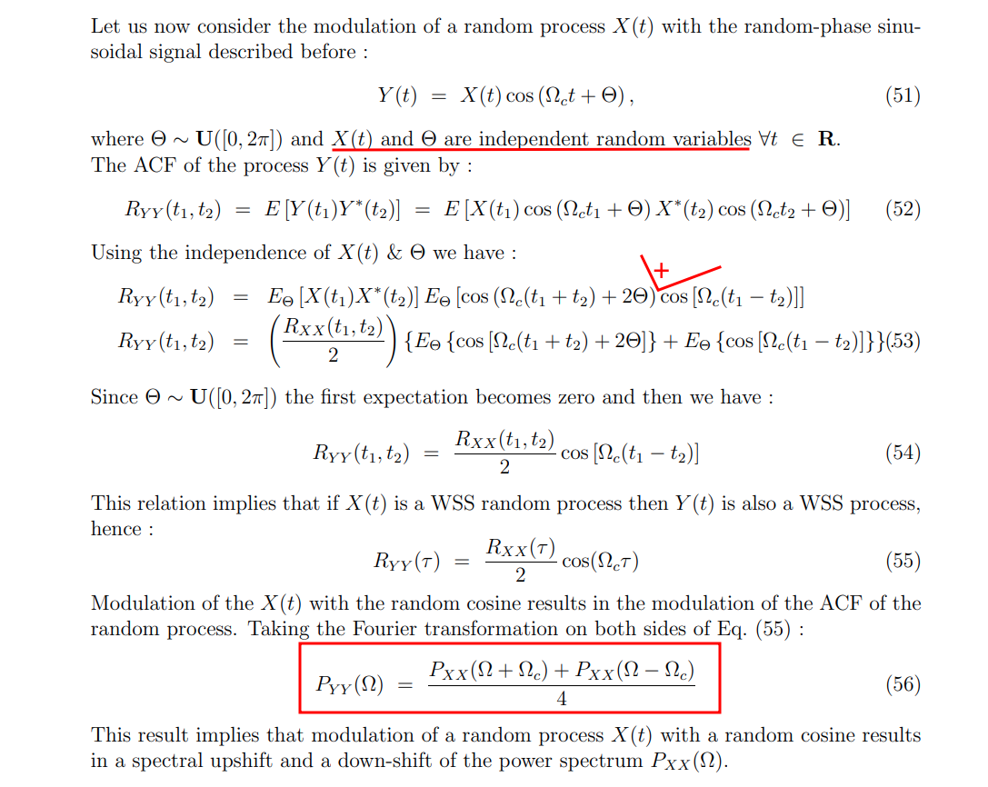
Modulation of WSS process

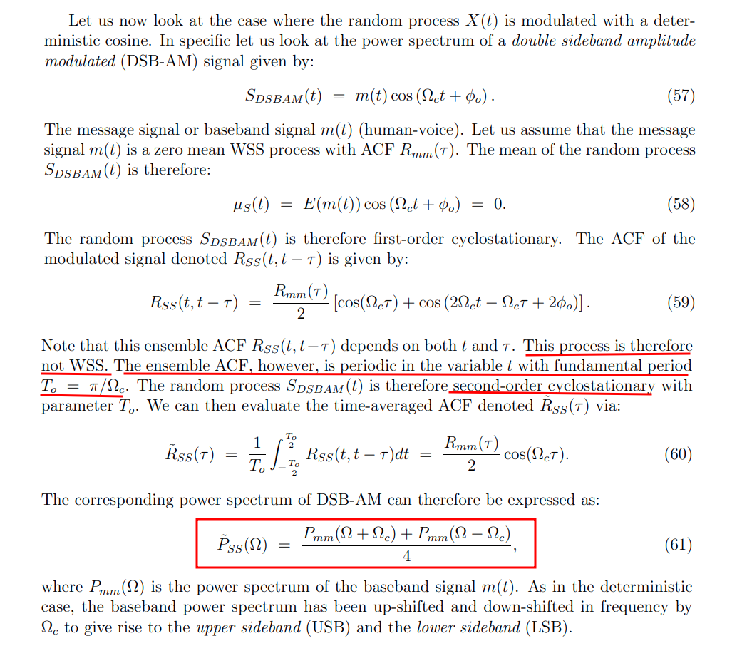
Balu Santhanam, Probability Theory & Stochastic Process 2020: Modulation of Random Processes

modulated with a random cosine

modulated with a deterministic cosine

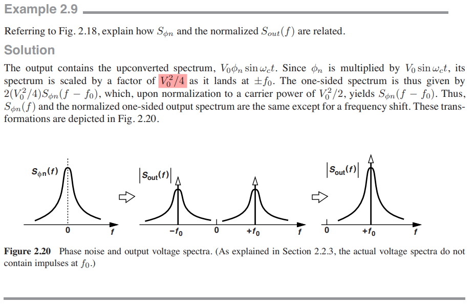
Hayder Radha, ECE 458 Communications Systems Laboratory Spring 2008: Lecture 7 - EE 179: Introduction to Communications - Winter 2006–2007 Energy and Power Spectral Density and Autocorrelation

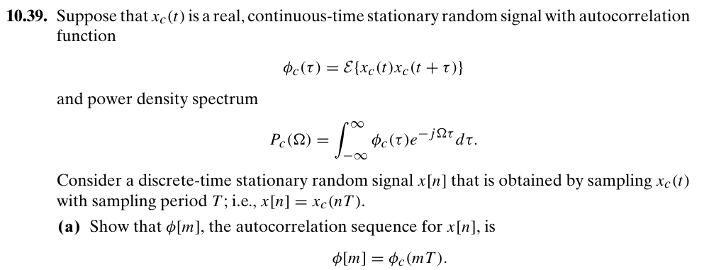
Sampling of WSS process

Balu Santhanam, Probability Theory & Stochastic Process 2020: Impulse sampling of Random Processes

DT sequence \(x[n]\)

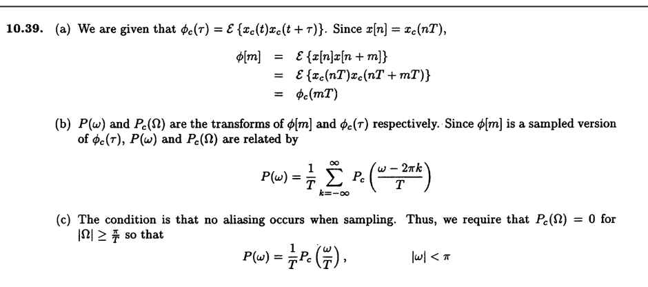
impulse train \(x_s(t)\)

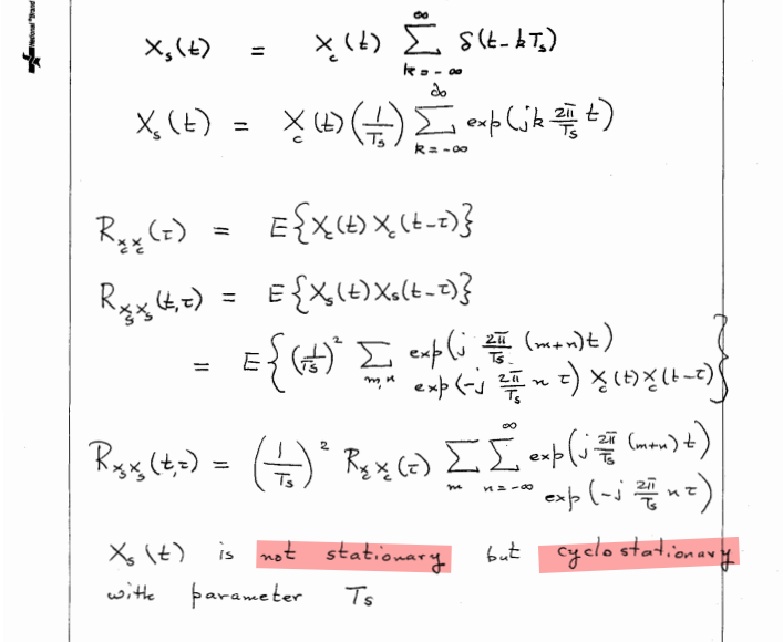
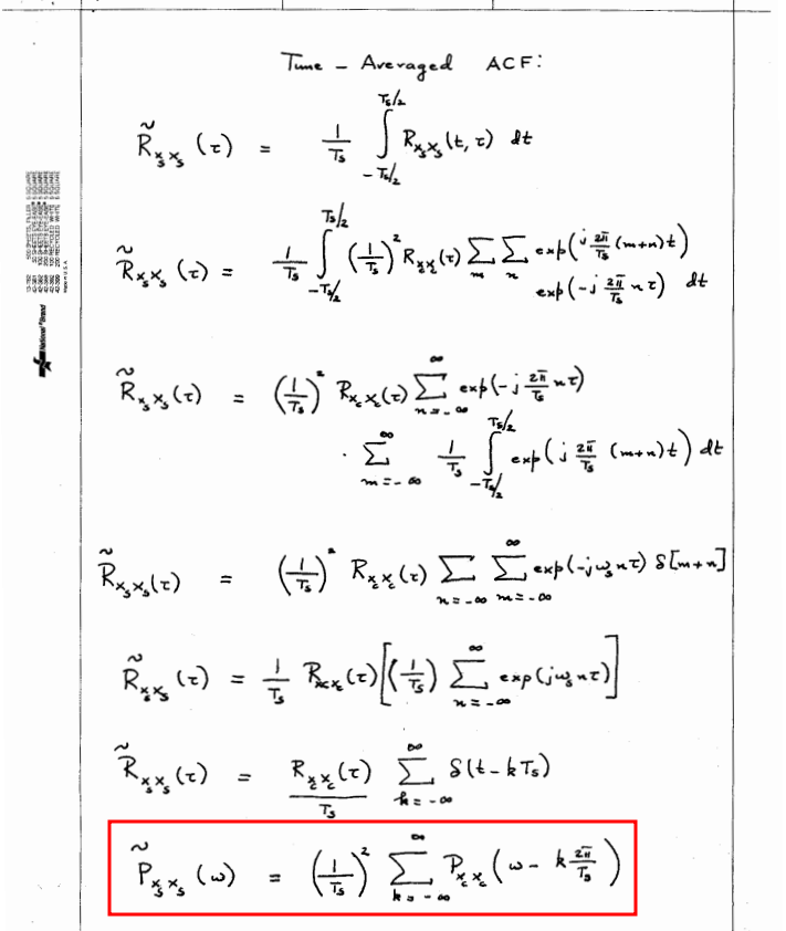
That is \[ P_{x_s x_s} (f)= \frac{1}{T_s^2}P_{xx}(f) \] where \(x[n]\) is sampled discrete-time sequence, \(x_s(t)\) is sampled impulse train

Noise Aliasing

apply foregoing observation

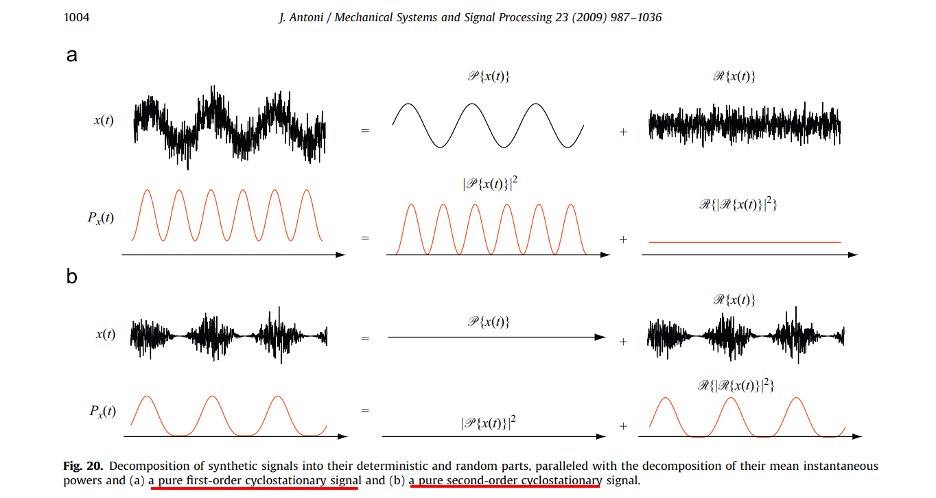
Cyclostationary Noise (Modulated Noise)

[https://ece-research.unm.edu/bsanthan/ece541/cyclo.pdf]

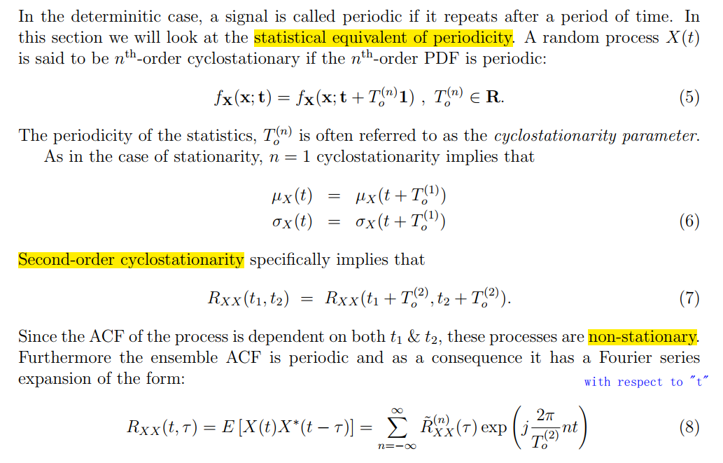
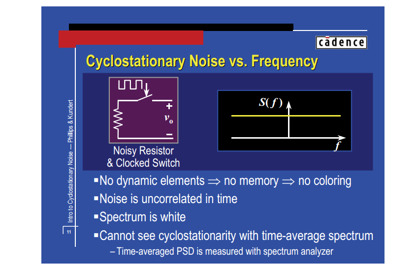
White Noise Modulation

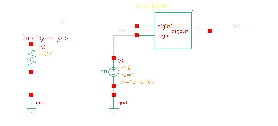
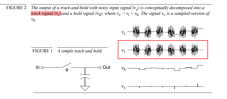
Noisy Resistor & Clocked Switch

\[ v_t (t) = v_i(t)\cdot m_t(t) \] where \(v_i(t)\) is input white noise, whose autocorrelation is \(A\delta(\tau)\), and \(m_t(t)\) is periodically operating switch, then autocorrelation of \(v_t(t)\) \[\begin{align} R_t (t_1, t_2) &= E[v_t(t_1)\cdot v_t(t_2)] \\ &= R_i(t_1, t_2)\cdot m_t(t_1)m_t(t_2) \end{align}\]

Then \[\begin{align} R_t(t, t-\tau) &= R_i(\tau)\cdot m_t(t)m_t(t-\tau) \\ & = A\delta(\tau) \cdot m_t(t)m_t(t-\tau) \\ & = A\delta(\tau) \cdot m_t(t) \end{align}\] Because \(m_t(t)=m_t(t+T)\), \(R_t(t, t-\tau)\) is is periodic in the variable \(t\) with period \(T\)

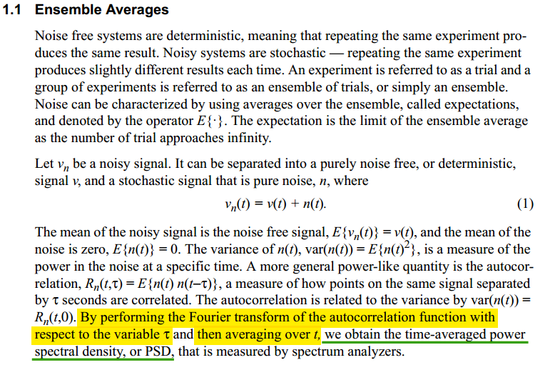
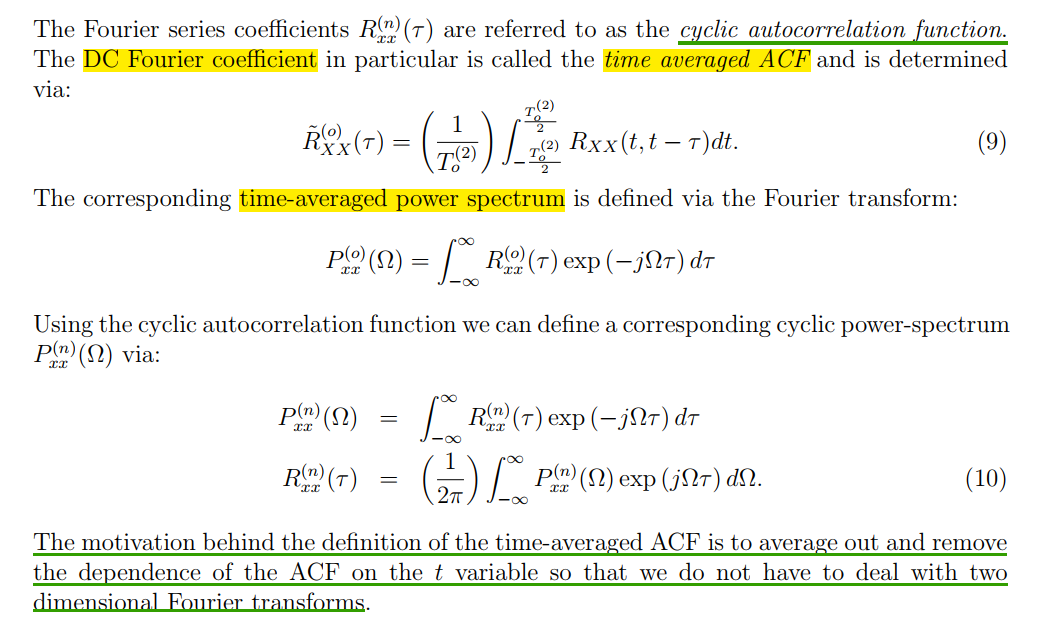
The time-averaged ACF is denoted as \(\tilde{R_t}(\tau)\)

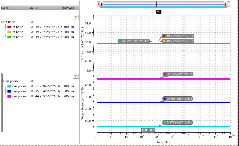
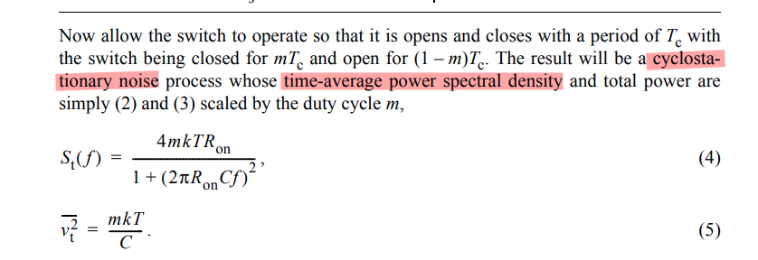
\[ \tilde{R}_{t}(\tau) = m\cdot A\delta(\tau) \] That is, \[ S_t(f) = m\cdot S_{A}(f) \]

Colored Noise Modulation

tavg_factor.drawio \[ \tilde{R_t}(\tau) = R_i(\tau)\cdot m_{tac}(\tau) \]

where \(m_t(t)m_t(t-\tau)\) averaged on \(t\) is denoted as \(m_{tac}(\tau)\) or \(\overline{m_t(t)m_t(t-\tau)}\)

The DC value of \(m_{tac}(\tau)\) can be calculated as below

for \(m\le 0.5\), the DC value of \(m_{tac}(\tau)\) \[ \frac{m\cdot mT}{T} = m^2 \]
for \(m\gt 0.5\), the DC value of \(m_{tac}(\tau)\) \[ \frac{(m+2m-1)(1-m)T + (2m-1)\{mT -(1-m)T\}}{T} = m^2 \]

Therefore, time-average power spectral density and total power are scaled by \(m^2\) in fundamental frequency sideband

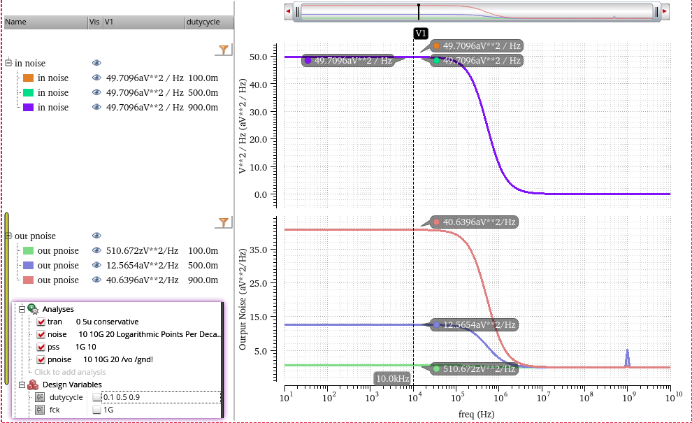
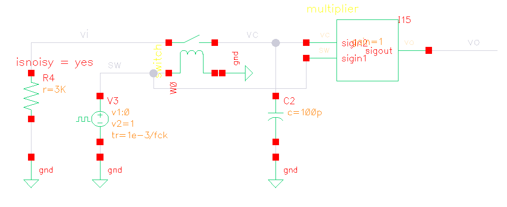
Switched-Capacitor Track signal

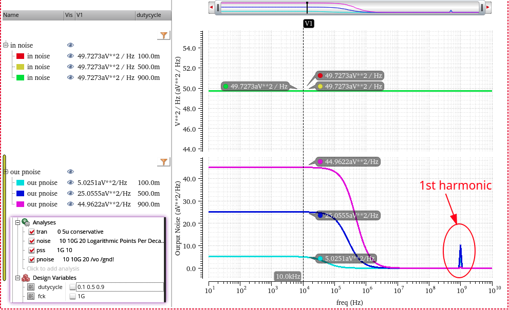
track signal pnoise (sc)

zoom in first harmonic by linear step of pnoise

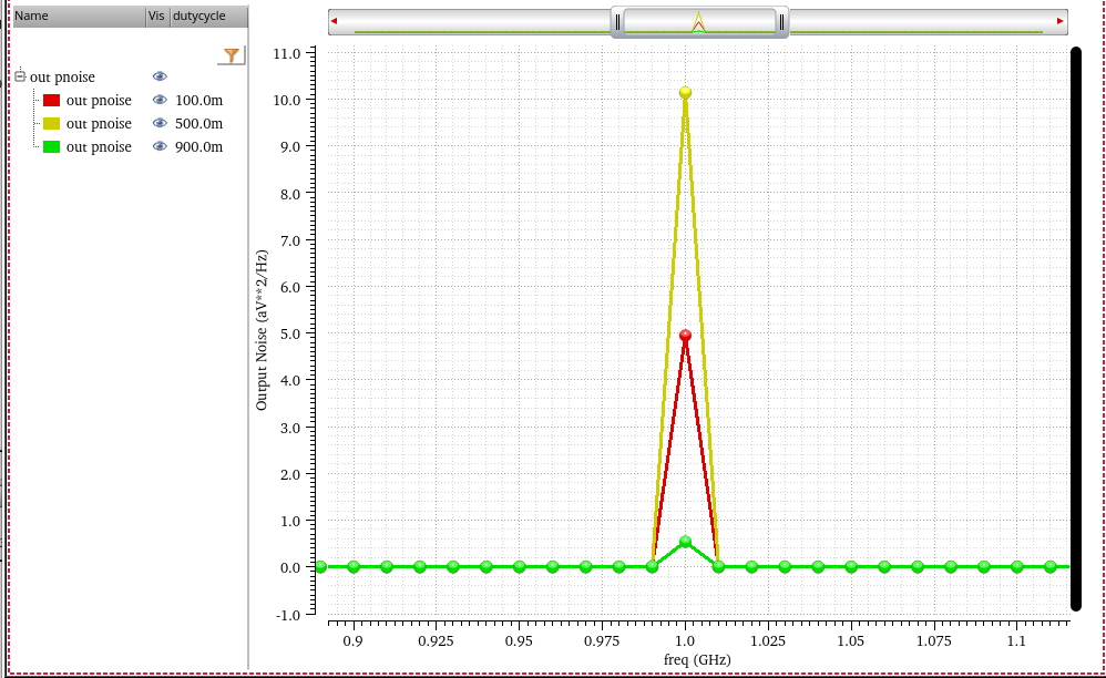
decreasing the rising/falling time of clock, the harmonics still retain

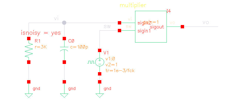
equivalent circuit for pnoise (eq)

thermal noise of R is modulated at first
then filtered by ideal filter

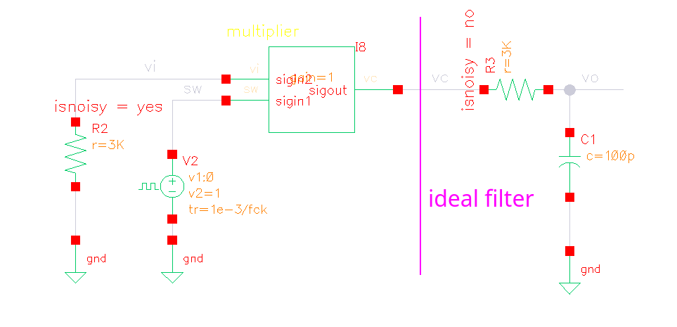
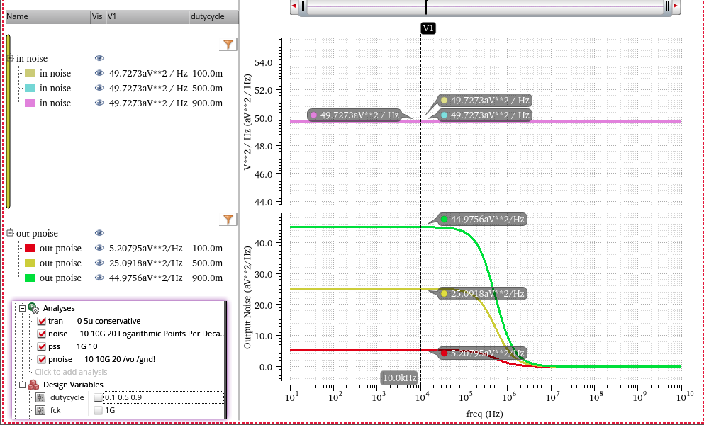
sc vs eq

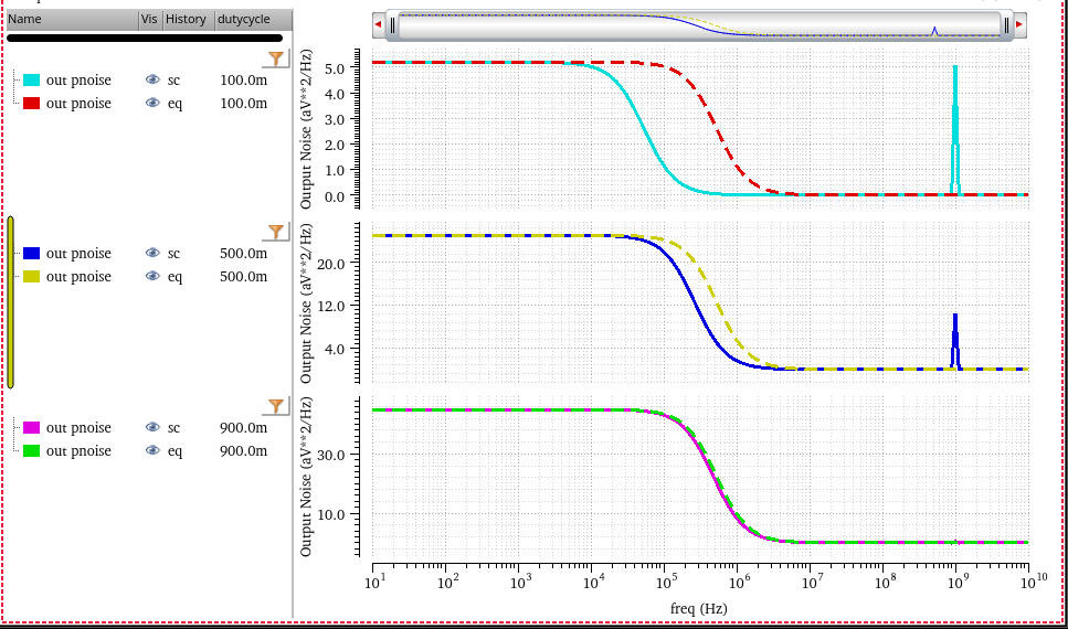
sc: harmonic distortion
eq: no harmonic distortion

Non-Stationary Processes

Wide-Sense-Stationary Noise

Much like sinusoidal-steady-state signal analysis, steady-state noise analysis methods assume an input x(t) of infinite duration, which is a Wide-Sense Stationary (WSS) random process

Frequency-domain Analysis

Time-domain Analysis

The output \(y(t)\) of a linear time-invariant (LTI) system \(h(t)\) \[\begin{align} R_{yy}(\tau) &= R_{xx}(\tau)*[h(\tau)*h(-\tau)] \\ &= S_{xx}(0)\delta(\tau) * [h(\tau)*h(-\tau)] \\ &= S_{xx}(0)[h(\tau)*h(-\tau)] \\ &= S_{xx}(0) \int_\alpha h(\alpha)h(\alpha-\tau)d\alpha \end{align}\]

with WSS white noise input \(x(t)\), \(R_{xx}(\tau)=S_{xx}(0)\delta(\tau)\), therefore

Non-stationary Noise

Assuming the noise applied duration is much less than the time constant, the output voltage does not reach steady-state and WSS noise analysis does not apply

In order to determine the response of an LTI system to a step noise input, the problem is more conveniently solved in the time-domain

input signal: step ramp input

noise current: step

Time-domain Analysis

The step noise input \(x(t) = \nu(t)u(t)\) \[ R_{xx}(t_1,t_2) = E[x(t_1)x(t_2)] = R_{\nu\nu}(t_1, t_2)u(t_1)u(t_2)=R_{\nu\nu}(t_1, t_2) \]

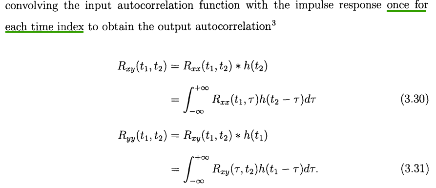
\[ R_{xy}(t_1, t_2) = E[x(t_1)y(t_2)] = E[x(t_1)(x(t_2)*h(t_2))] = E(x(t_1)x(t_2))*h(t_2) = R_{xx}(t_1,t_2)*h(t_2) \]

\[ R_{yy}(t_1,t_2) = E[y(t_1)y(t_2)] = E[(x(t_1)*h(t_1))y(t_2)] = E[x(t_1)y(t_2)]*h(t_1)=R_{xy}(t_1,t_2)*h(t_1) \]

the absolute value of each time index is important for a non-stationary signal, and only the time difference was important for WSS signals

\[\begin{align} R_{yy}(t_1,t_2) &= h(t_1)*R_{\nu\nu}(t_1, t_2)*h(t_2) \\ &= h(t_1)*S_{xx}(0)\delta(t_2-t_1)*h(t_2) \\ &=S_{xx}(0) h(t_1)*(\delta(t_2-t_1)*h(t_2)) \\ &= S_{xx}(0)h(t_1)*h(t_2-t_1) \\ &= S_{xx}(0)\int_\tau h(\tau)h(t_2-t_1+\tau))d\tau \end{align}\]

That is \[ \sigma^2_y (t)= R_{yy}(t_1,t_2)|_{t_1=t_2=t}=S_{xx}(0)\int_{-\infty}^t |h(\tau)|^2d\tau \]

\(t\), the upper limit of integration is just intuitive, which lacks strict derivation

Because stable systems have impulse responses that decay to zero as time goes to infinity, the output noise variance approaches the WSS result as time approaches infinity

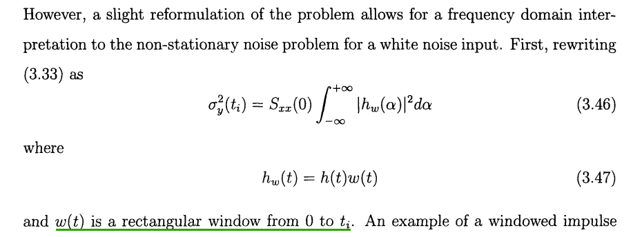
Frequency-domain Analysis

Because the definition of the PSD assumes that the variance of the noise process is independent of time, the PSD of a non-stationary process is not very meaningful

Input Referred Noise

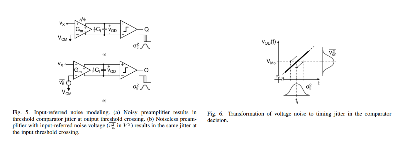
Noise Voltage to Timing Jitter Conversion & noise gain

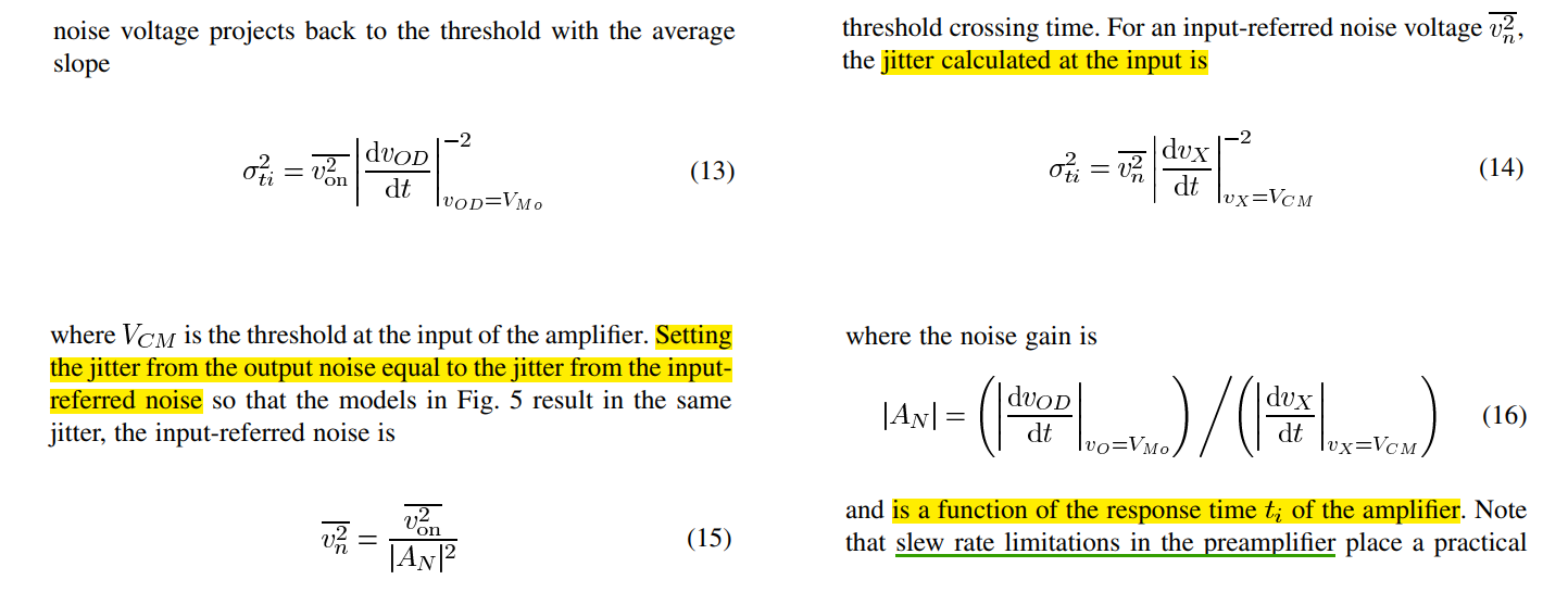
with a step ramp input \(v_X(t) = Mtu(t)\)

The noise gain is \[ |A_N(t_i)| = A_0 (1-e^{t_i/\tau_o})u(t) \] where \(t_i\) is crossing time of ideal threshold comparator
\[\begin{align} \overline{v_n^2} &= \frac{\overline{v_{on}^2}}{|A_N|^2} \\ &= \frac{G_n}{G_m}\frac{kT}{C}\frac{1}{A_0}\frac{1+e^{-t_i/\tau_o}}{1-e^{-t_i/\tau_o}} \\ &=4kT\frac{G_n}{G_m^2}\frac{1}{4R_oC} \coth(\frac{t_i}{2\tau_o}) \\ &= 4kTR_n\frac{1}{4\tau_o} \coth(\frac{t_i}{2\tau_o}) \end{align}\]

where \(R_n = \frac{G_n}{G_m^2}\), the equivalent thermal noise resistance

reference

Alan V Oppenheim, Ronald W. Schafer. Discrete-Time Signal Processing, 3rd edition [pdf]

R. E. Ziemer and W. H. Tranter, Principles of Communications, 7th ed., Wiley, 2013 [pdf]

John G. Proakis and Masoud Salehi, Fundamentals of communication systems 2nd ed [pdf]

Rhee, W. and Yu, Z., 2024. Phase-Locked Loops: System Perspectives and Circuit Design Aspects. John Wiley & Sons

Phillips, Joel R. and Kenneth S. Kundert. "Noise in mixers, oscillators, samplers, and logic: an introduction to cyclostationary noise." Proceedings of the IEEE 2000 Custom Integrated Circuits Conference. [pdf, slides]

Antoni, J., "Cyclostationarity by examples", Mechanical Systems and Signal Processing, vol. 23, no. 4, pp. 987–1036, 2009 [https://docente.unife.it/docenti/dleglc/a-a-2010-2011-dmsm/ciclostazionarieta.pdf]

Kundert, Ken. (2006). Simulating Switched-Capacitor Filters with SpectreRF. URL:https://designers-guide.org/analysis/sc-filters.pdf

STEADY-STATE AND CYCLO-STATIONARY RTS NOISE IN MOSFETS [https://ris.utwente.nl/ws/portalfiles/portal/6038220/thesis-Kolhatkar.pdf]

Christian-Charles Enz. "High precision CMOS micropower amplifiers" [pdf]

T. Sepke, P. Holloway, C. G. Sodini and H. -S. Lee, "Noise Analysis for Comparator-Based Circuits," in IEEE Transactions on Circuits and Systems I: Regular Papers, vol. 56, no. 3, pp. 541-553, March 2009 [https://dspace.mit.edu/bitstream/handle/1721.1/61660/Speke-2009-Noise%20Analysis%20for%20Comparator-Based%20Circuits.pdf]

Sepke, Todd. "Comparator design and analysis for comparator-based switched-capacitor circuits." (2006). [https://dspace.mit.edu/handle/1721.1/38925]