LC Oscillator
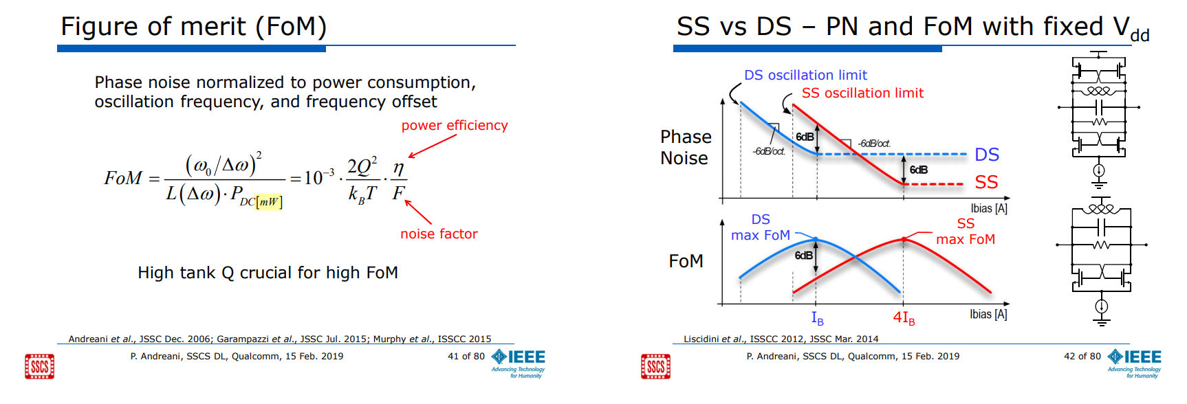
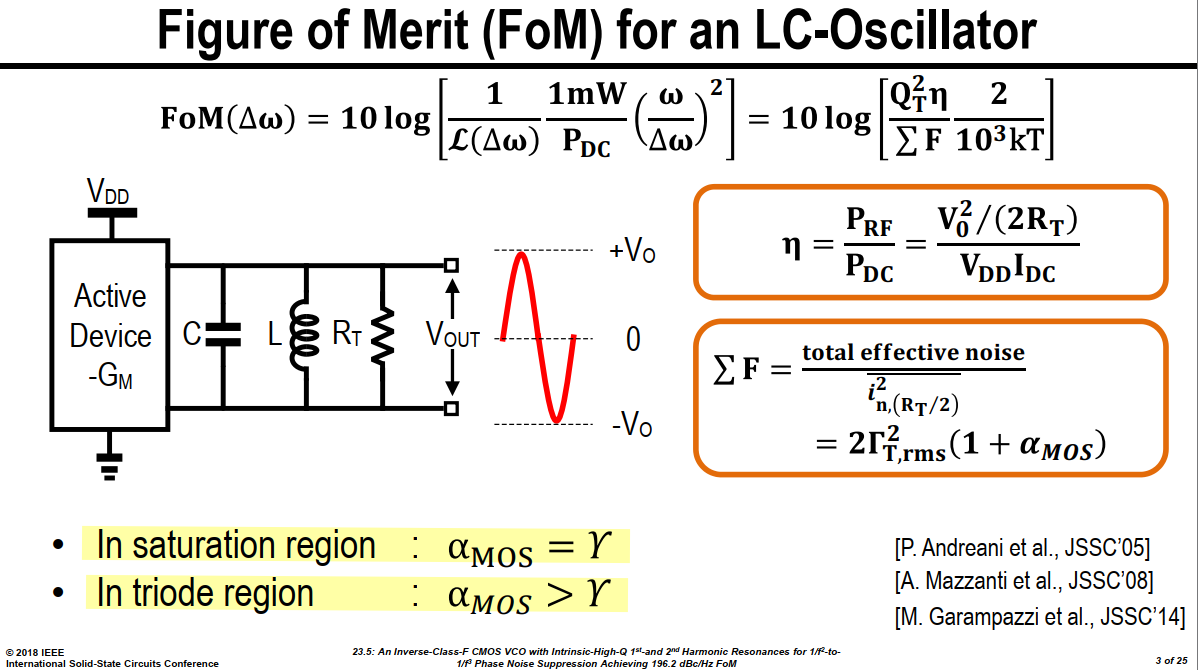
Figure of Merit (FoM)
M. Garampazzi et al., "An Intuitive Analysis of Phase Noise Fundamental Limits Suitable for Benchmarking LC Oscillators," in IEEE Journal of Solid-State Circuits, vol. 49, no. 3, pp. 635-645, March 2014 [https://sci-hub.jp/10.1109/JSSC.2014.2301760]
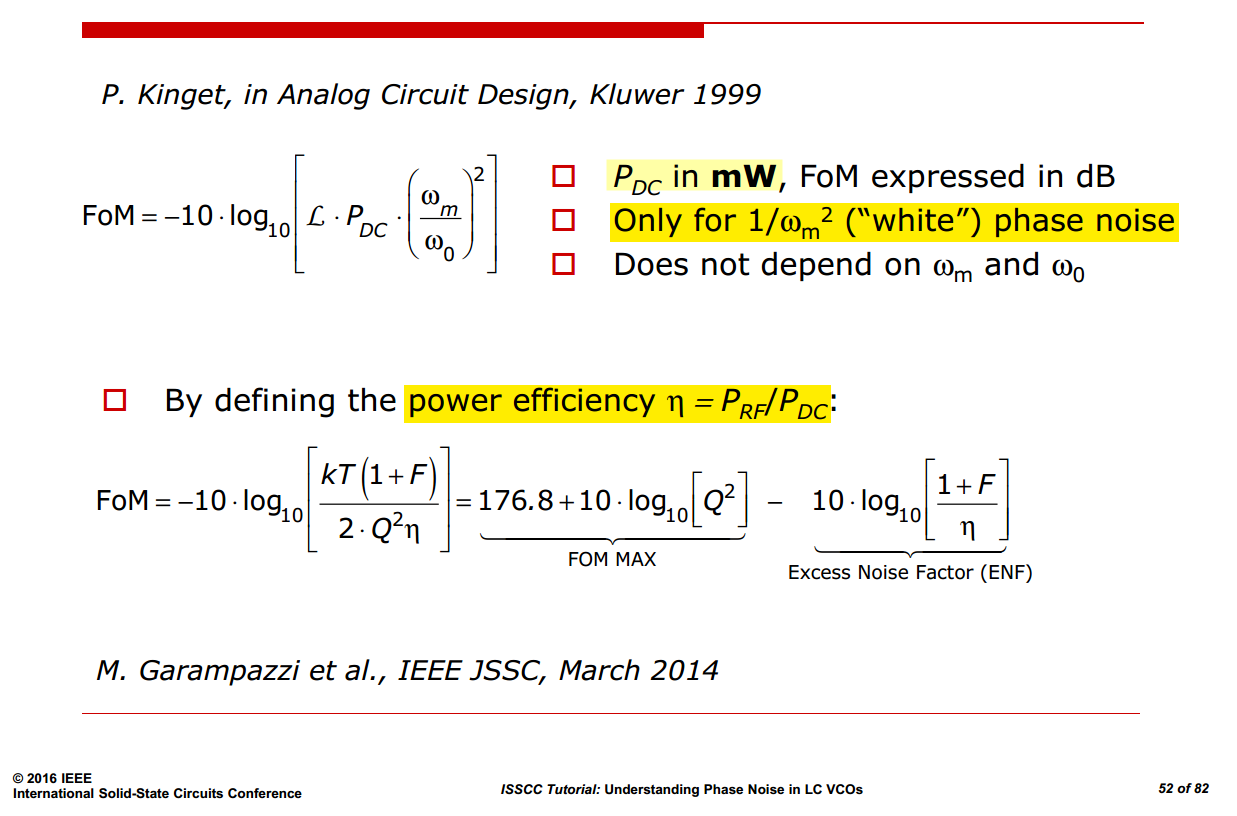
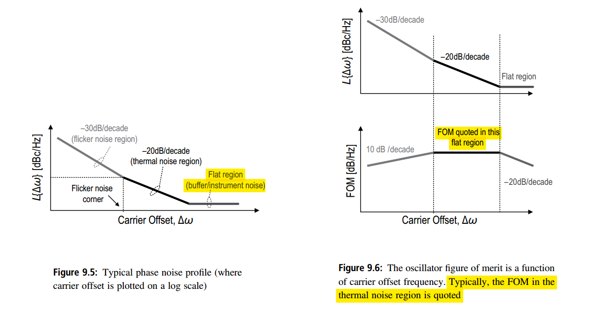
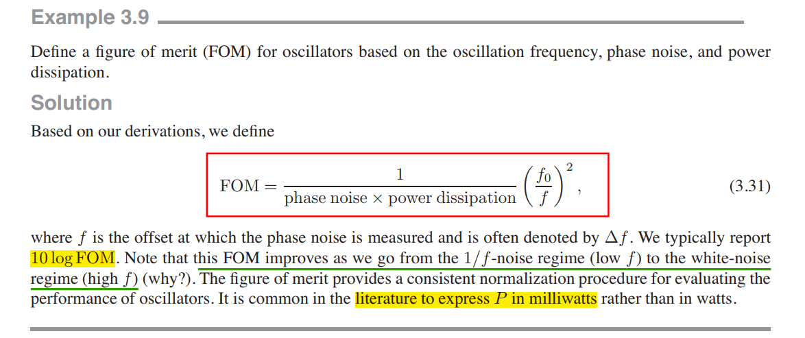
In general, FOM varies with carrier offset, but when reported as a single number it is assumed that FOM was calculated using measurements from the thermal noise region where the FOM plateaus
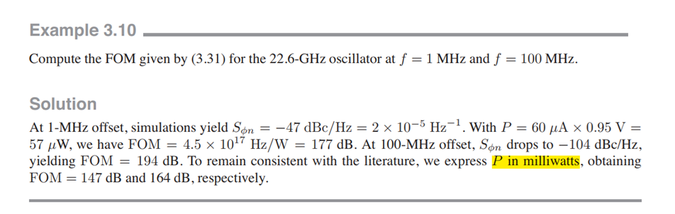
1 | Sphi_1M = -47; % dBc/Hz |
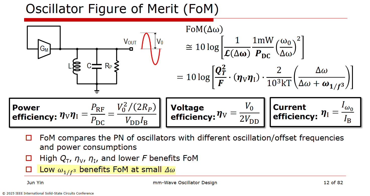 \[
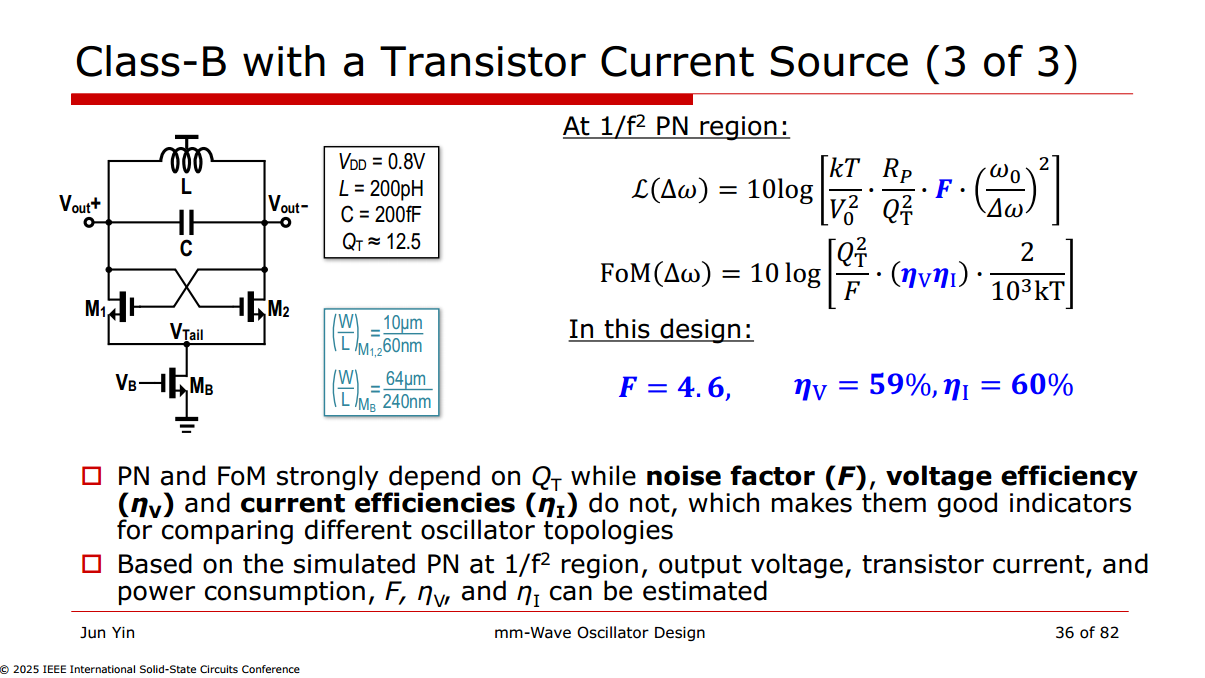
\boxed{\eta = \frac{V_0^2/(2R_P)}{V_{DD} I_B} = \frac{V_0}{2V_{DD}}
\frac{V_0}{R_P I_B}=\frac{V_0}{2V_{DD}} \frac{I_{\omega_0}}{I_B}=\eta_V
\eta_I}
\]
\[
\boxed{\eta = \frac{V_0^2/(2R_P)}{V_{DD} I_B} = \frac{V_0}{2V_{DD}}
\frac{V_0}{R_P I_B}=\frac{V_0}{2V_{DD}} \frac{I_{\omega_0}}{I_B}=\eta_V
\eta_I}
\]
1 | kB= 1.380649e-23; T=300; |
LC Oscillator Structures
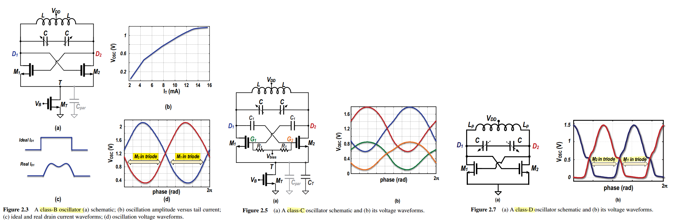
Class-C CMOS Oscillator
A. Mazzanti and P. Andreani, "Class-C Harmonic CMOS VCOs, With a General Result on Phase Noise," in IEEE Journal of Solid-State Circuits, vol. 43, no. 12, pp. 2716-2729, Dec. 2008 [https://sci-hub.ru/10.1109/JSSC.2008.2004867]
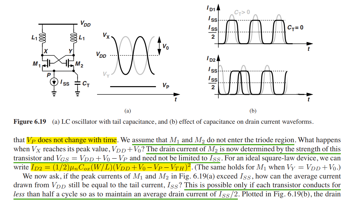
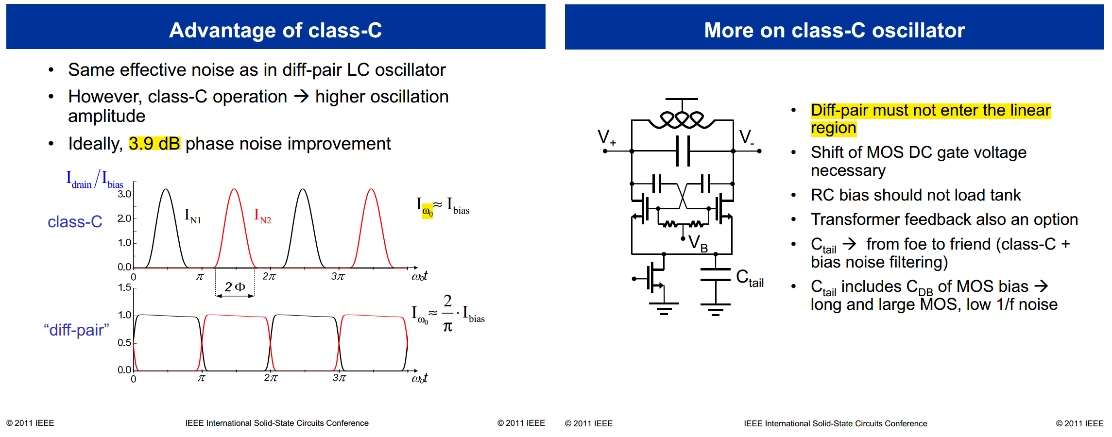
Tail Current-Shaping Technique
B. Soltanian and P. Kinget, "A tail current-shaping technique to reduce phase noise in LC VCOs," Proceedings of the IEEE 2005 Custom Integrated Circuits Conference, 2005., San Jose, CA, USA, 2005 [https://sci-hub.ru/10.1109/CICC.2005.1568734]
—, "Tail Current-Shaping to Improve Phase Noise in LC Voltage-Controlled Oscillators," in IEEE Journal of Solid-State Circuits, vol. 41, no. 8, pp. 1792-1802, Aug. 2006 [https://sci-hub.ru/10.1109/JSSC.2006.877273]
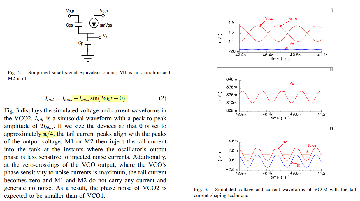
Assuming cross-coupled pair act as ideal swithes and tail current waveform in \(I_\text{tail}=1-\cos 2\omega_0 t\)
\[ x(t)= \begin{cases} 1+\cos(2\omega_0 t), & -\pi < 2\omega_0 t < \pi,\\[2mm] 0, & \pi < 2\omega_0 t < 3\pi. \end{cases} \]
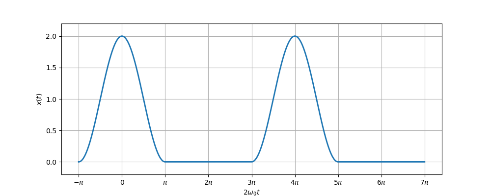
\[ \boxed{x(t) = 1 +\textcolor{red}{\frac{8}{3\pi}\cos(\omega_0 t)} +\frac{1}{2}\cos(2\omega_0 t) -\frac{8}{15\pi}\cos(3\omega_0 t) +\cdots} \]
The fundamental harmonic coefficients is \(\frac{8}{3\pi}\) and we know class-B coeff. is \(\frac{2}{\pi}\)
Class-D CMOS Oscillator
L. Fanori and P. Andreani, "A 2.5-to-3.3GHz CMOS Class-D VCO," 2013 IEEE International Solid-State Circuits Conference Digest of Technical Papers, San Francisco, CA, USA, 2013 [https://sci-hub.red/10.1109/ISSCC.2013.6487763]
—, "Class-D CMOS Oscillators," in IEEE Journal of Solid-State Circuits, vol. 48, no. 12, pp. 3105-3119, Dec. 2013 [https://sci-hub.red/10.1109/JSSC.2013.2271531]
—, "A Class-D CMOS DCO with an on-chip LDO," ESSCIRC 2014 - 40th European Solid State Circuits Conference (ESSCIRC), Venice Lido, Italy, 2014 [https://sci-hub.red/10.1109/ESSCIRC.2014.6942090]
TODO 📅
| Class-B | Class-D | |
|---|---|---|
| oscillation amplitude | Idd & LC-tank losses | VDD |
| current consumption | VDD & LC-tank losses |
Class-F CMOS Oscillator
Huijung Kim, Seonghan Ryu, Yujin Chung, Jinsung Choi and Bumman Kim, "A low phase-noise CMOS VCO with harmonic tuned LC tank," in IEEE Transactions on Microwave Theory and Techniques, vol. 54, no. 7, pp. 2917-2924, July 2006 [https://sci-hub.ru/10.1109/tmtt.2006.877439]
M. Babaie and R. B. Staszewski, "Third-harmonic injection technique applied to a 5.87-to-7.56GHz 65nm CMOS Class-F oscillator with 192dBc/Hz FOM," 2013 IEEE International Solid-State Circuits Conference Digest of Technical Papers, San Francisco, CA, USA, 2013 [https://sci-hub.ru/10.1109/ISSCC.2013.6487764]
—, "A Class-F CMOS Oscillator," in IEEE Journal of Solid-State Circuits, vol. 48, no. 12, pp. 3120-3133, Dec. 2013 [https://ieeexplore.ieee.org/stamp/stamp.jsp?tp=&arnumber=6576263]
TODO 📅
Class-F2 CMOS Oscillator
TODO 📅
Class-F3 CMOS Oscillator
TODO 📅
Class-F23 CMOS Oscillator
TODO 📅
Class-F-1 CMOS Oscillator
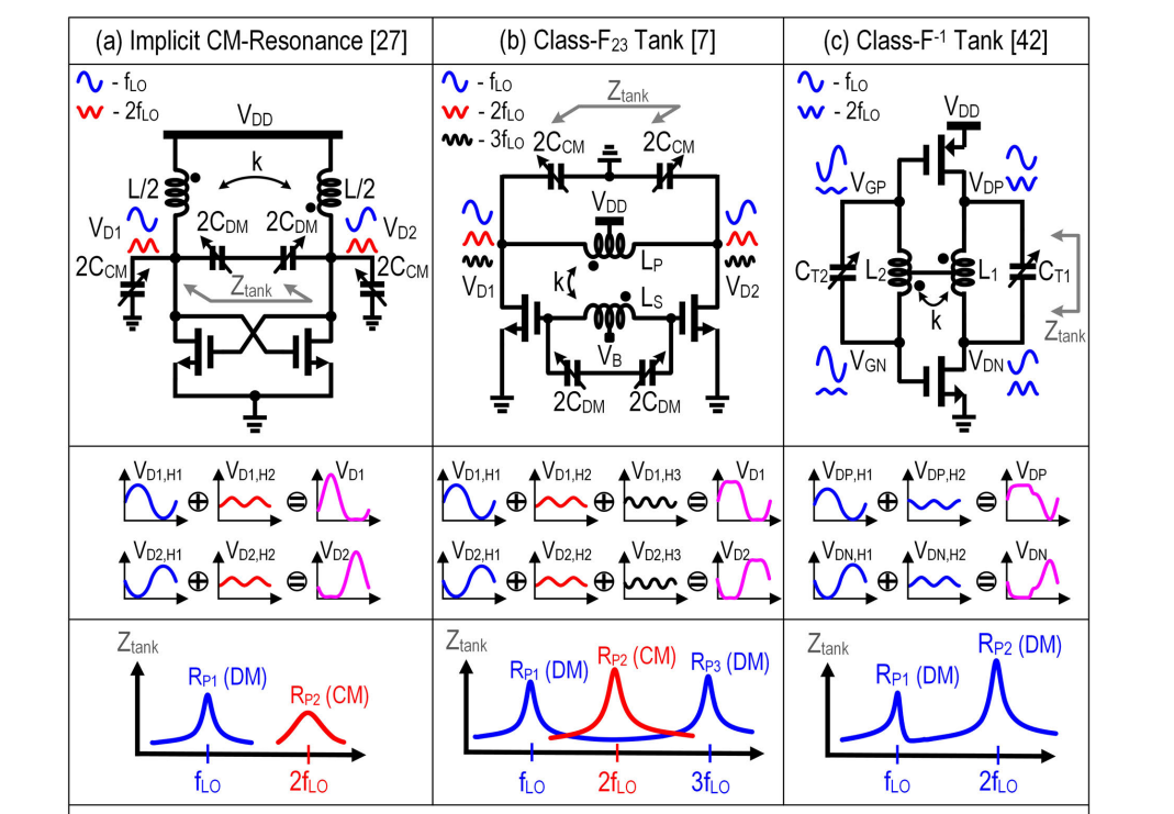
C. -C. Lim, J. Yin, P. -I. Mak, H. Ramiah and R. P. Martins, "An inverse-class-F CMOS VCO with intrinsic-high-Q 1st- and 2nd-harmonic resonances for 1/f2-to-1/f3 phase-noise suppression achieving 196.2dBc/Hz FOM," 2018 IEEE International Solid-State Circuits Conference - (ISSCC), San Francisco, CA, USA, 2018 [paper]
—, "An Inverse-Class-F CMOS Oscillator With Intrinsic-High-Q First Harmonic and Second Harmonic Resonances," in IEEE Journal of Solid-State Circuits, vol. 53, no. 12, pp. 3528-3539, Dec. 2018 [https://sci-hub.jp/10.1109/JSSC.2018.2875099]
X. Meng, H. Li, P. Chen, J. Yin, P. -I. Mak and R. P. Martins, "Analysis and Design of a 15.2-to-18.2-GHz Inverse-Class-F VCO With a Balanced Dual-Core Topology Suppressing the Flicker Noise Upconversion," in IEEE Transactions on Circuits and Systems I: Regular Papers, vol. 70, no. 12, pp. 5110-5123, Dec. 2023
TODO 📅
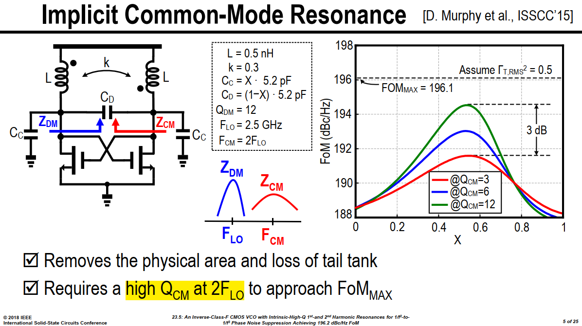
Higher \(Q_\text{CM}\) is preferred for better FoM
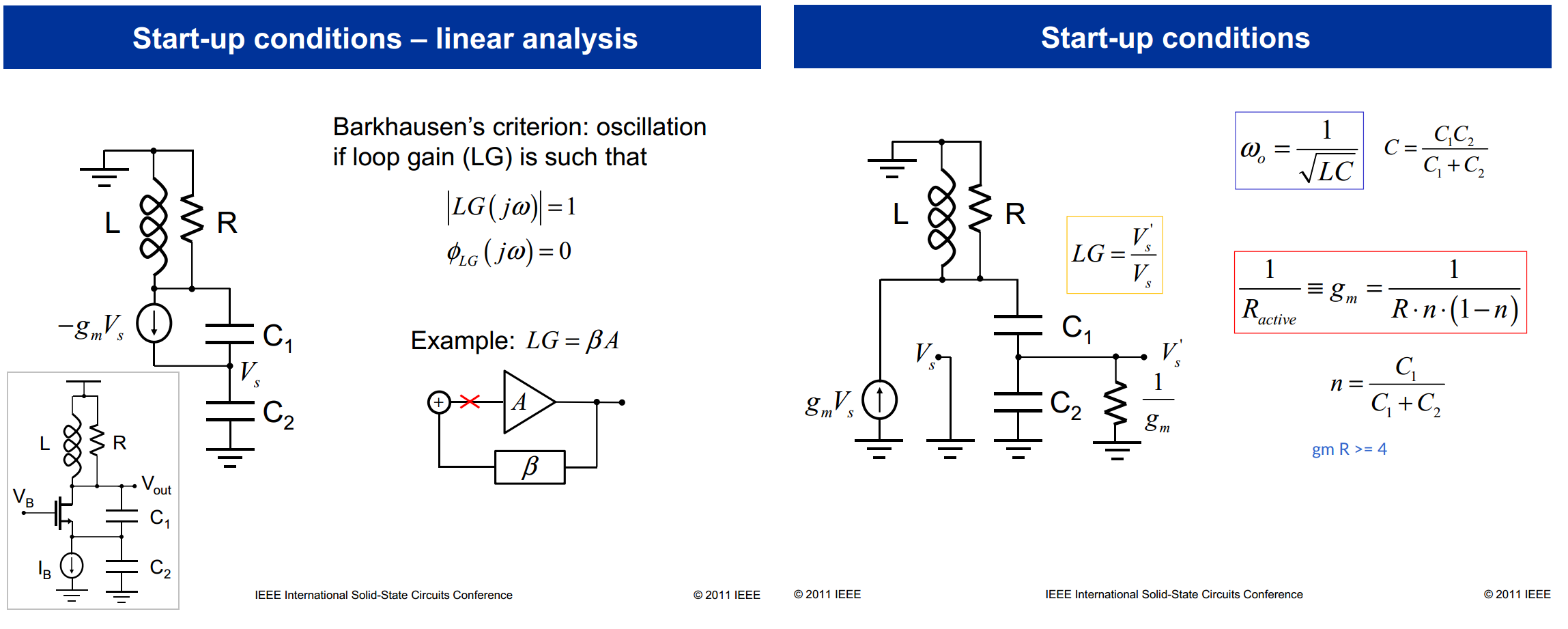
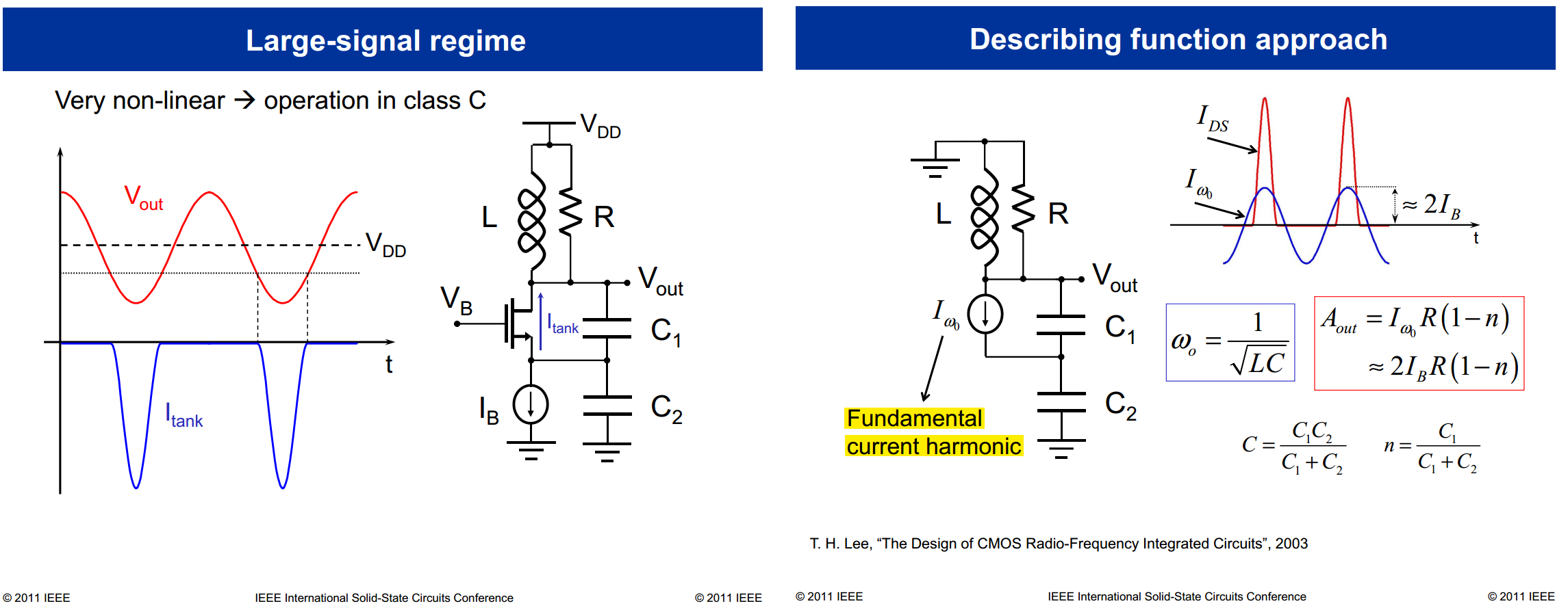
Colpitts oscillator
John Rogers, Calvin Plett, and Foster Dai. 2006. Integrated Circuit Design for High-Speed Frequency Synthesis (Artech House Microwave Library). Artech House, Inc., USA.
Jri Lee, "Communication Integrated Circuits.", [https://cc.ee.ntu.edu.tw/~jrilee/publications/Comm_IC.pdf]
Start-up conditions \[ \boxed{g_mR_p \geq 4} \]
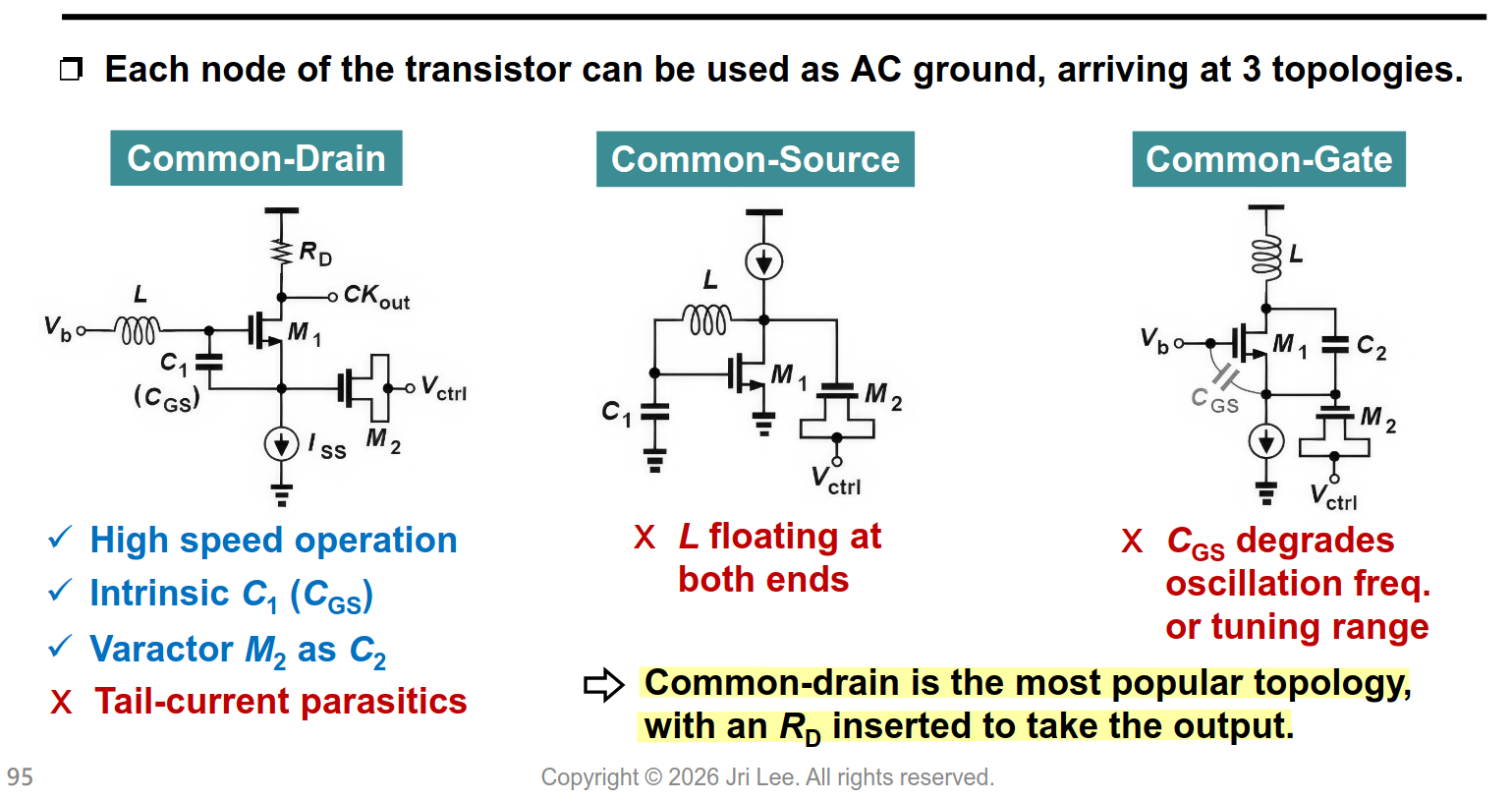
This type of oscillator could be operated with only one transistor. In modern times, the abundance of transistors and the desire for differential circuits favors a symmetric Colpitts oscillators
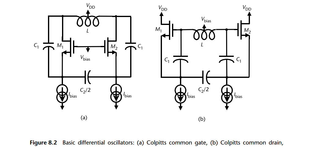
common-source Colpitts
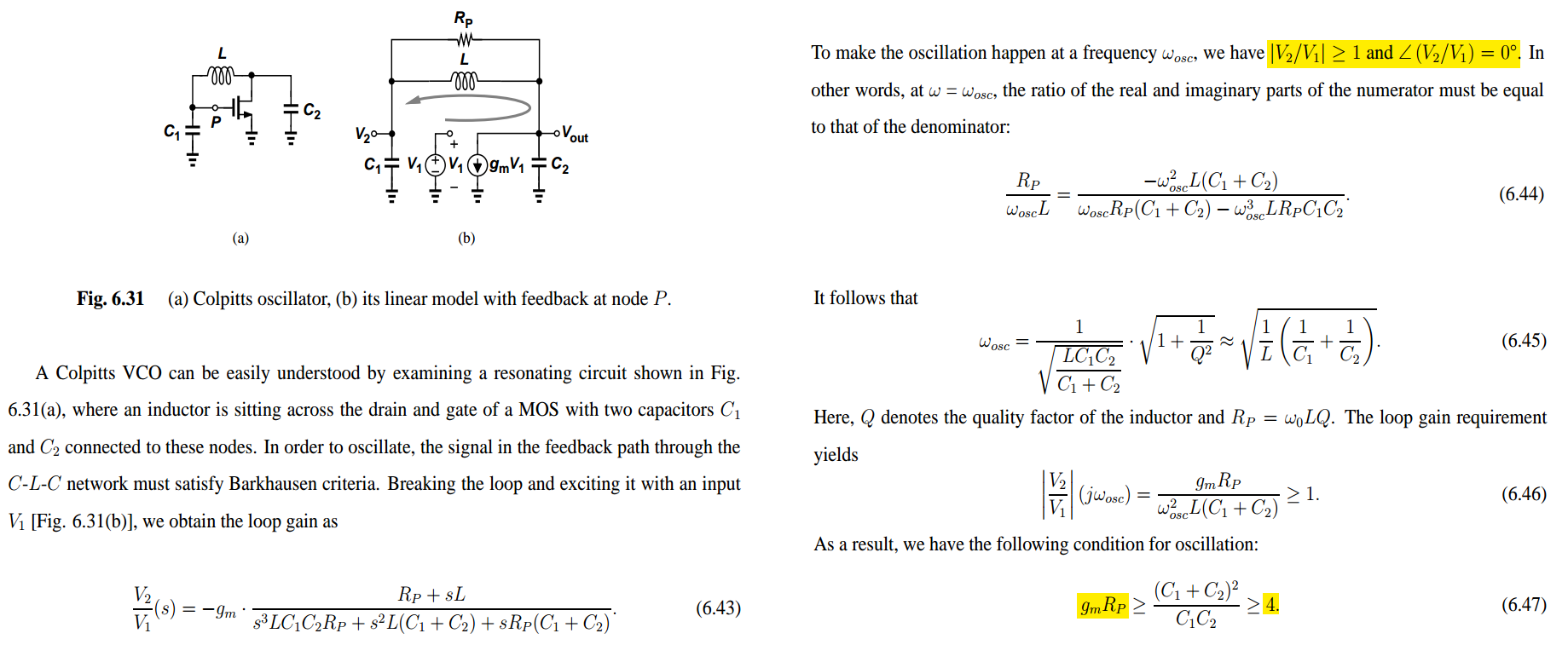
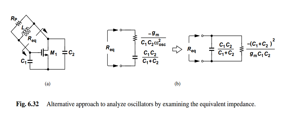
common-gate Colpitts
TODO 📅
Class-B Oscillators
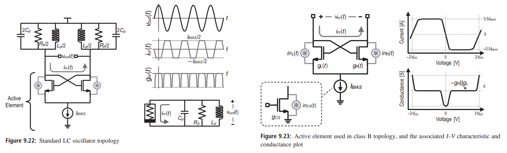
active element provides a negative conductance only when the input voltage is small
For larger voltages, one of the transistors in the differential pair will be off, while the other will be on, and the conductance drops to zero
Output Amplitude
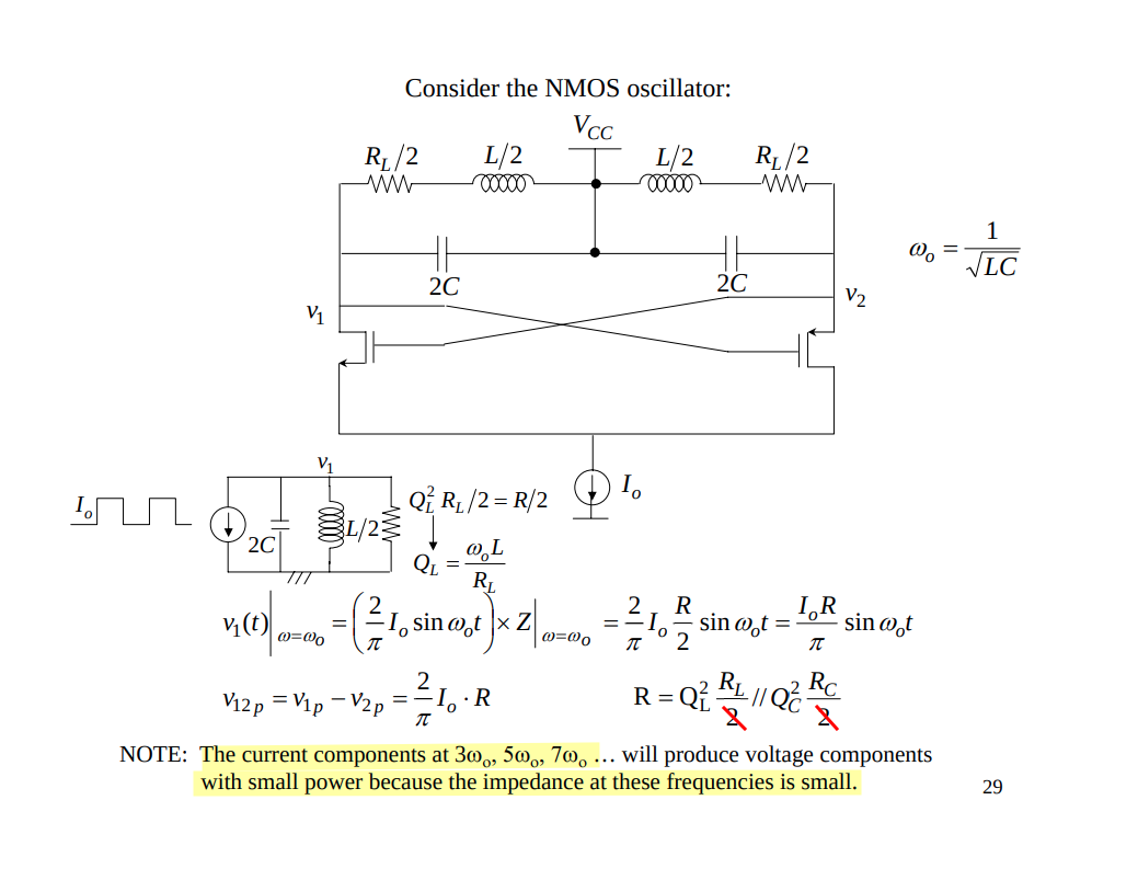
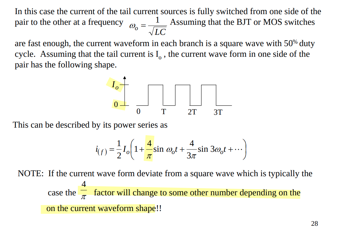
Edgar Sanchez-Sinencio. ECEN 665, OSCILLATORS [https://people.engr.tamu.edu/s-sanchez/665%20Oscillators.pdf]
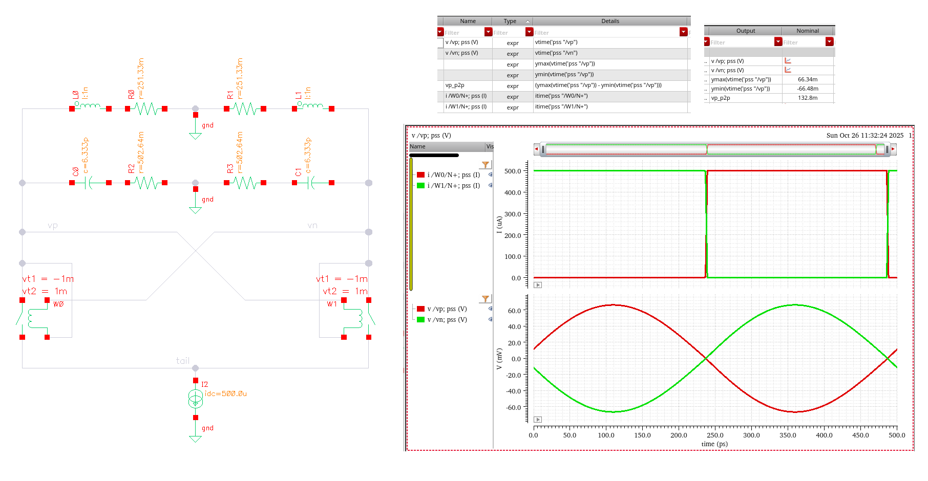
NMOS Realization — single pair
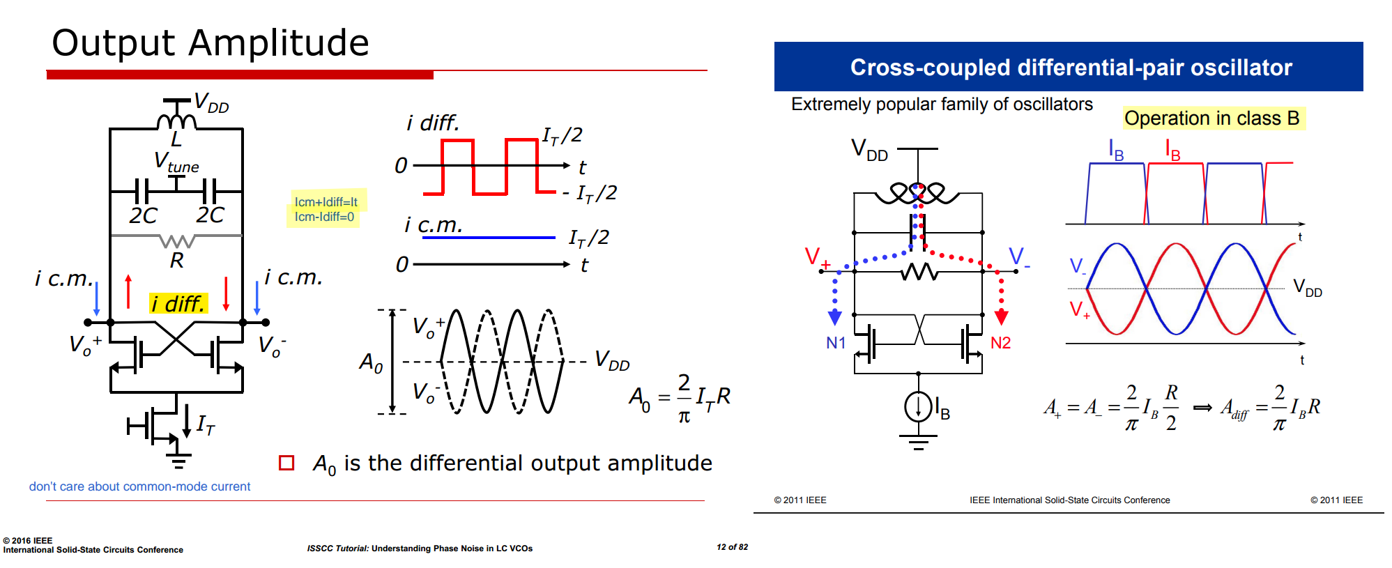
common mode current don't contribute to output amplitude
1 | L0 = 1e-9 * 2; |
CMOS Realization — double pair
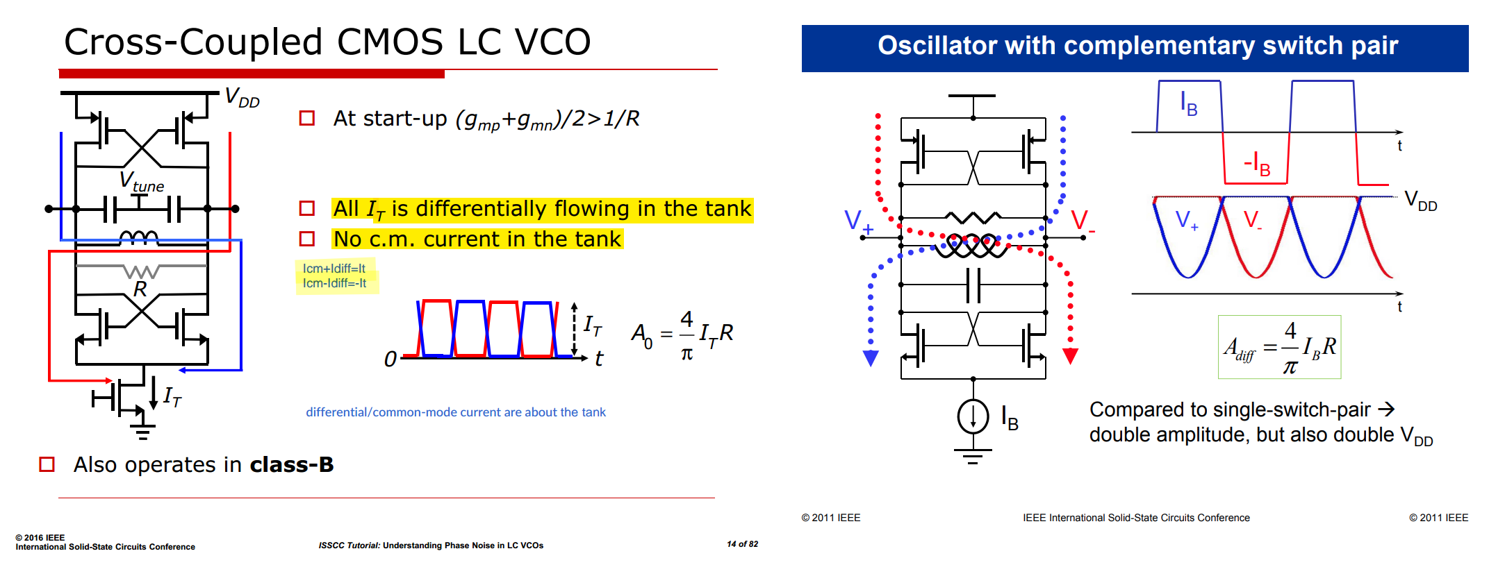
Owing to switch-off PMOS eliminating common mode current, all \(I_T\) is differentially flowing in the tank
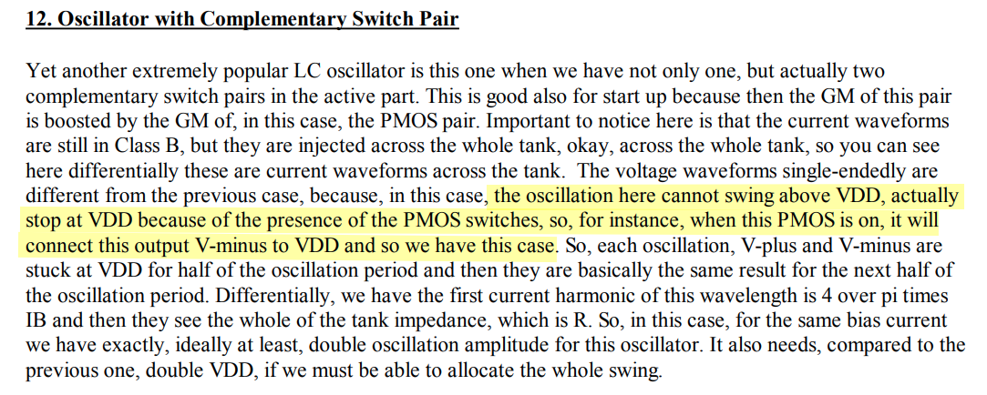

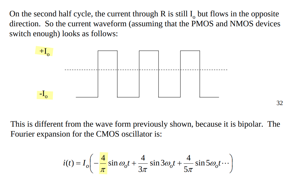
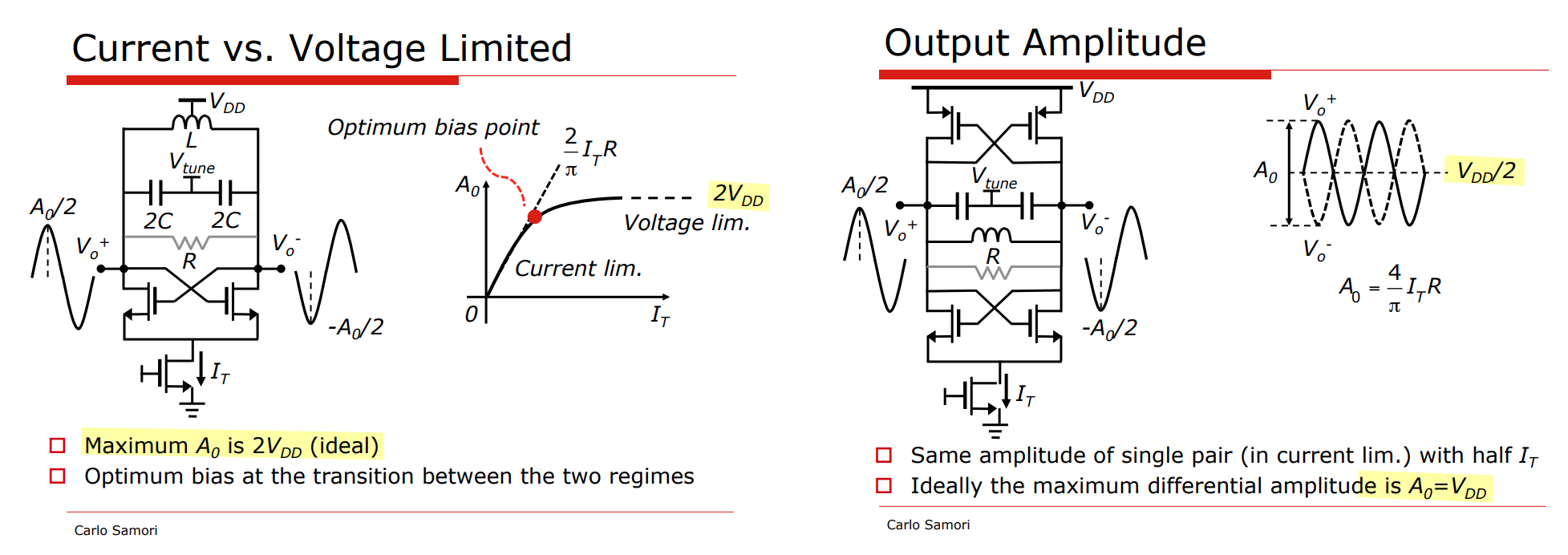
current vs voltage limited
Luong, H. C., & Yin, J. (2016). Transformer-based design techniques for oscillators and frequency dividers. Springer International Publishing
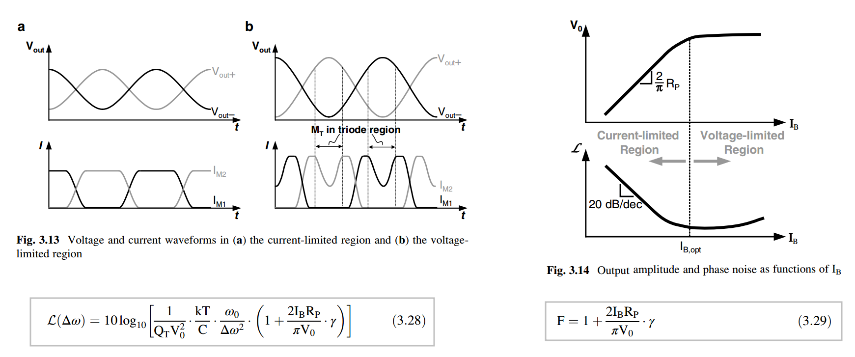
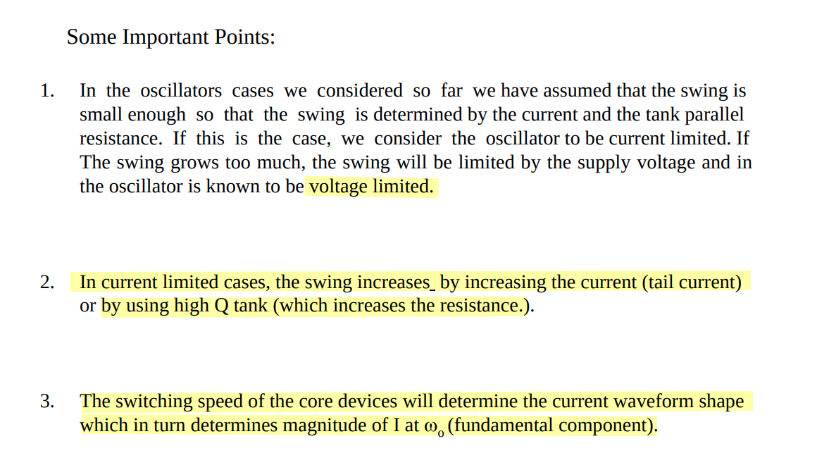
Once the swing clips near the supply (voltage-limited regime), more tail current just burns power and can even hurt phase noise
Class-B Power/Current Efficiency
Z. Wang, S. Diao, L. He, X. Jiang and F. Lin, "Analysis of Current Efficiency for CMOS Class-B LC Oscillators," in IEEE Transactions on Circuits and Systems I: Regular Papers, vol. 62, no. 5, pp. 1345-1352, May 2015 [https://sci-hub.jp/10.1109/TCSI.2015.2411792]
L. Bertulessi, S. Levantino and C. Samori, "Analysis of power efficiency in high-performance class-B oscillators," 2016 12th Conference on Ph.D. Research in Microelectronics and Electronics (PRIME), Lisbon, Portugal, 2016 [https://sci-hub.jp/10.1109/PRIME.2016.7519525]
TODO 📅
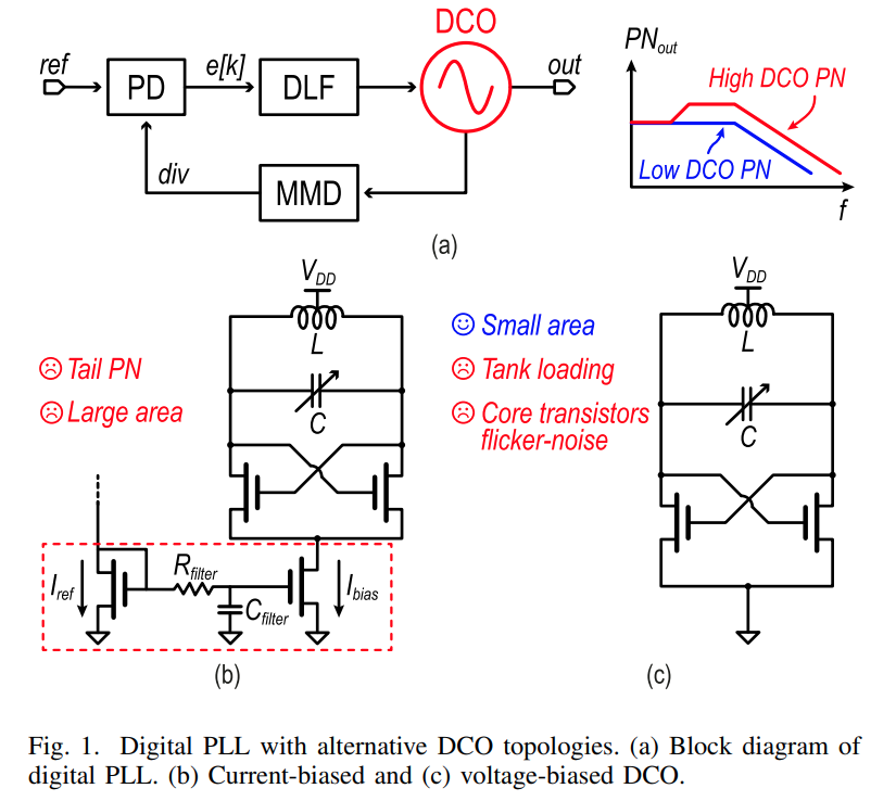
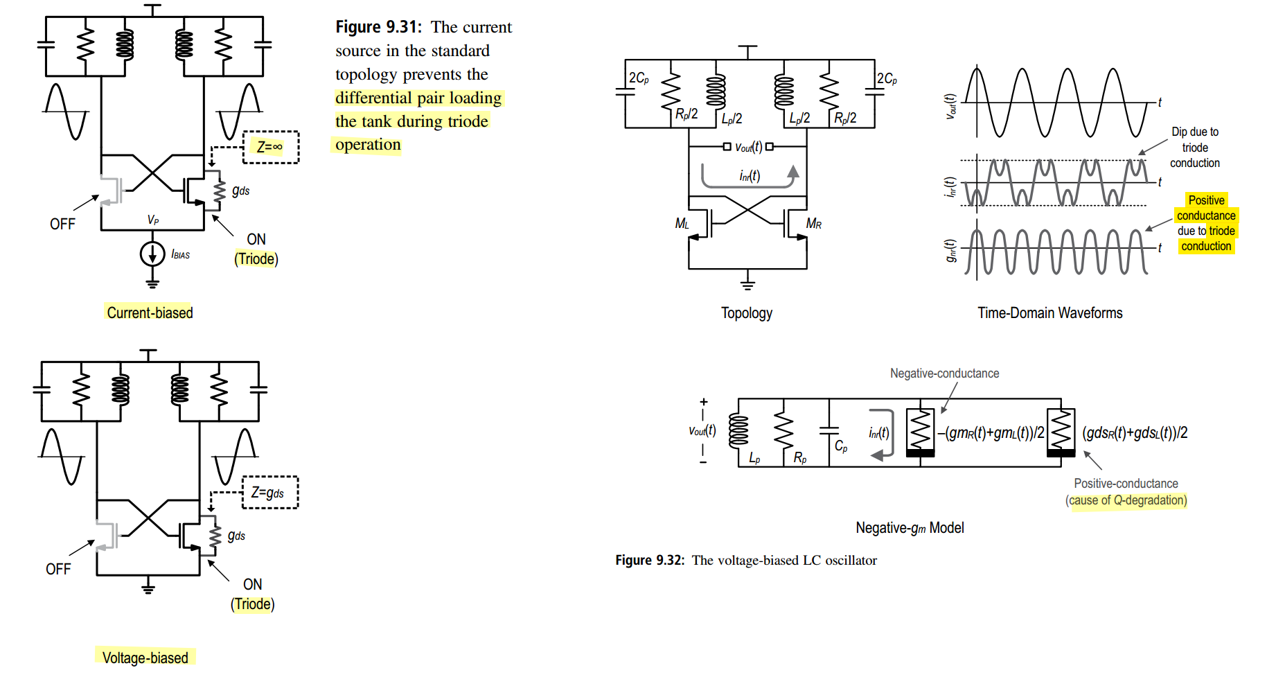
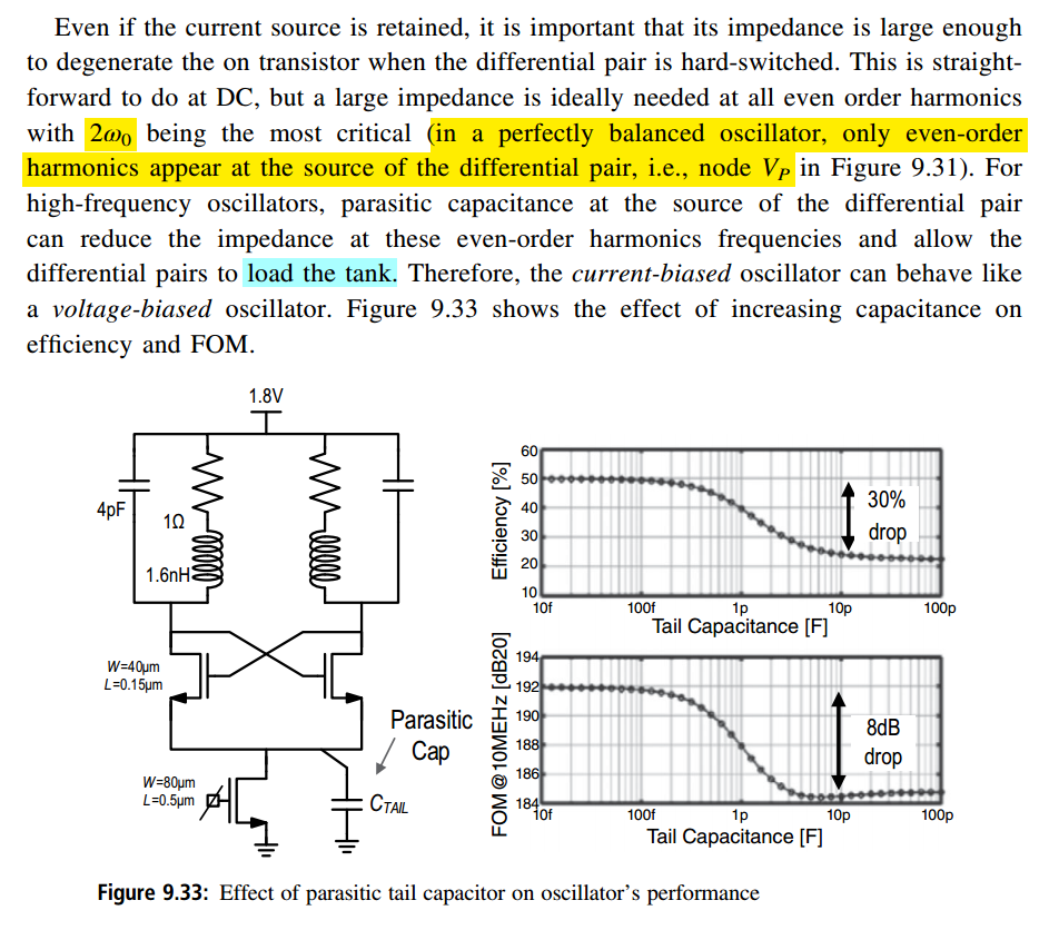
Current-biased & voltage-biased
S. Gallucci et al., "A Low-Noise Digital PLL With an Adaptive Common-Mode Resonance Tuning Technique for Voltage-Biased Oscillators," in IEEE Journal of Solid-State Circuits, vol. 60, no. 12, pp. 4572-4586, Dec. 2025
TODO 📅
Startup & Geff
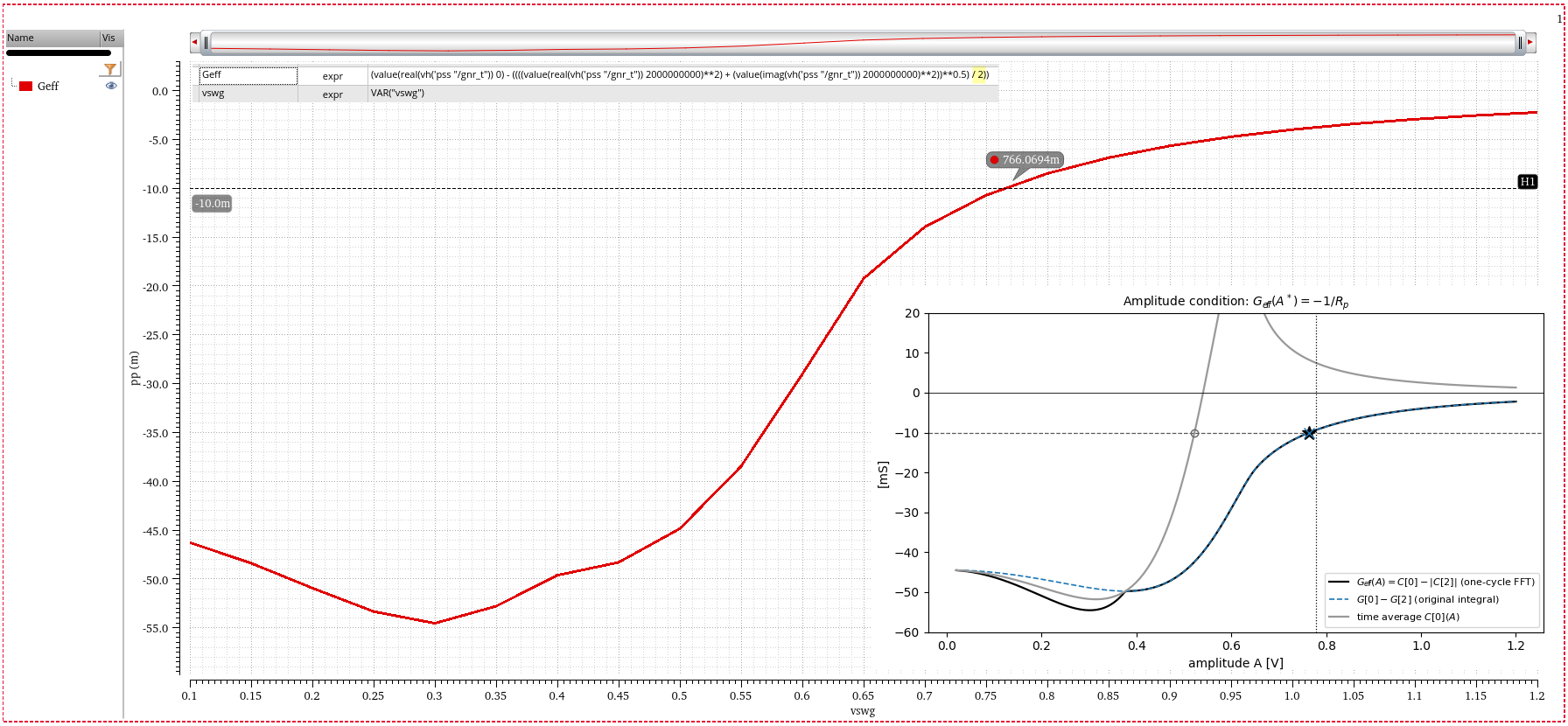
effective or large signal conductance
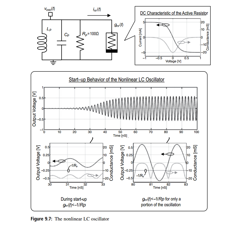
Note that the gnr frequency is twice of oscillator voltage frequency
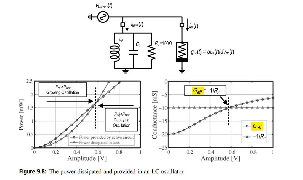
Power Conservation Requirements
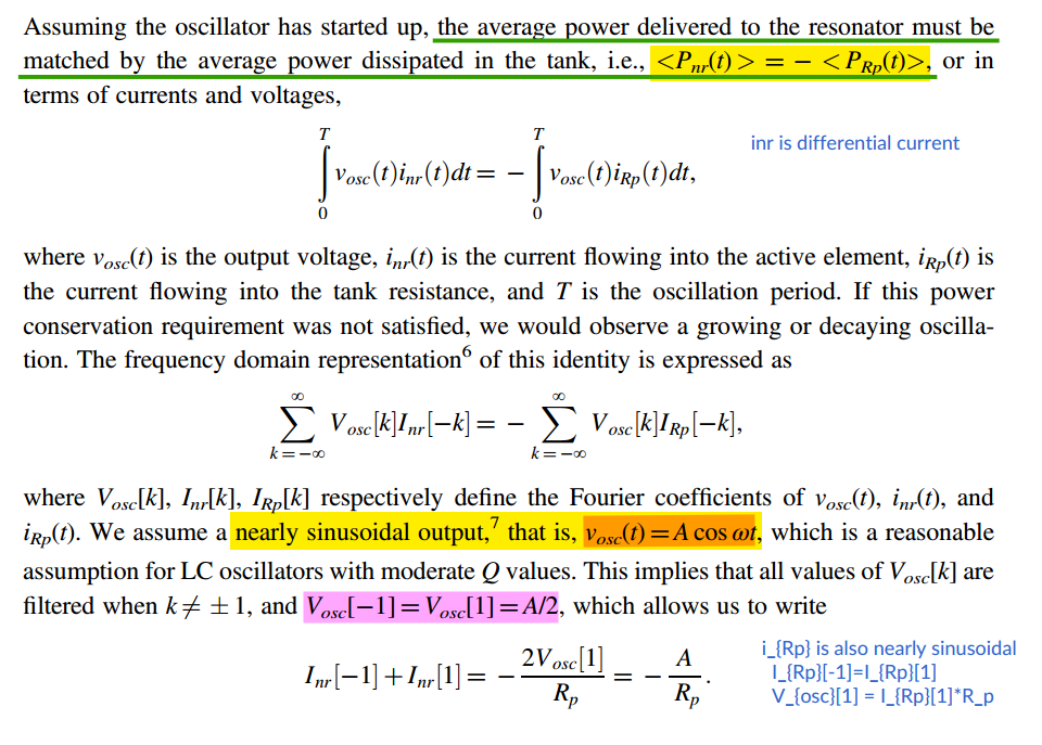
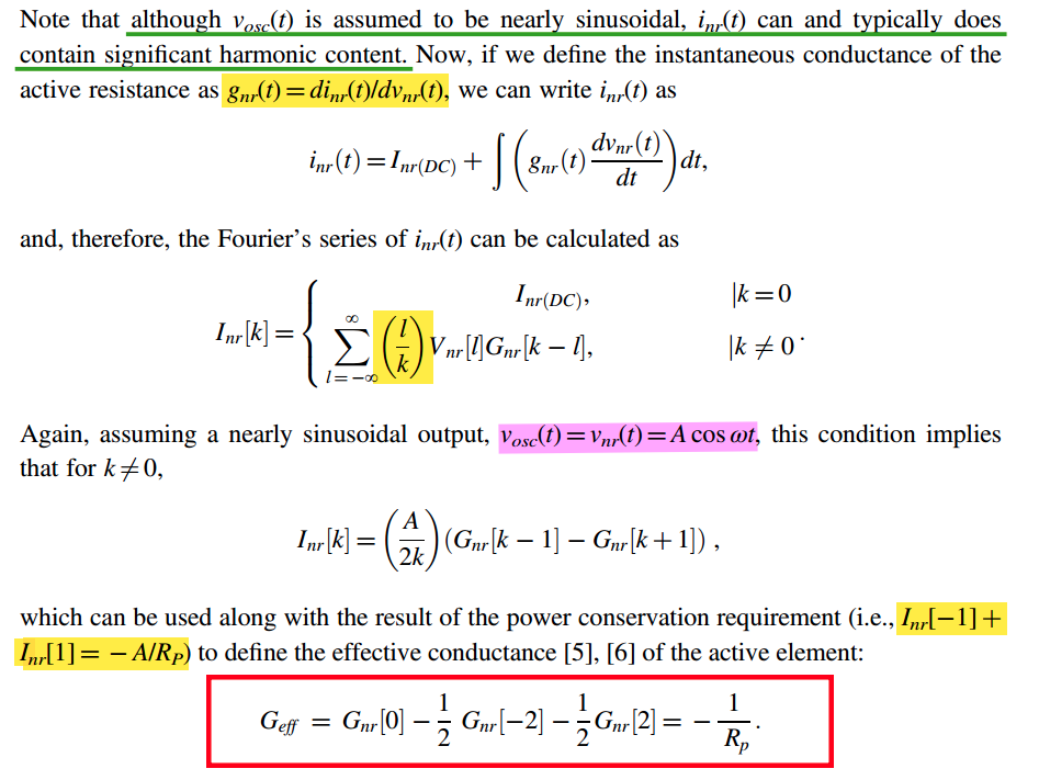
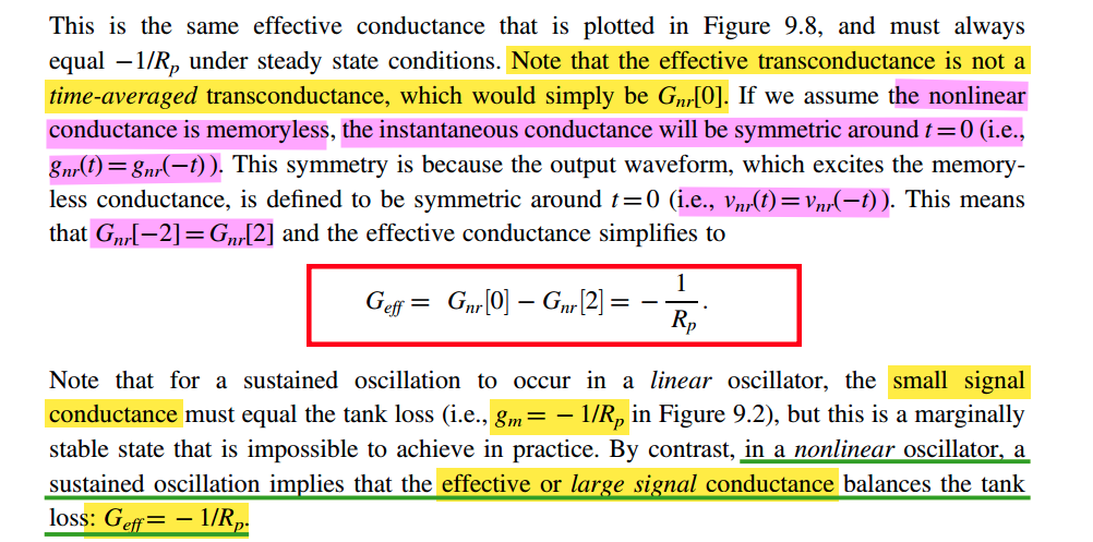
Since the Fourier transform of a real and even function is also real and even, the derivation above assumes that \(V_{\text{osc}}(t)\) is real and even, which implies that \(g_{\text{nr}}(t)\) is likewise real and even — \(G_\text{nr}\) is real and even
1 |
|
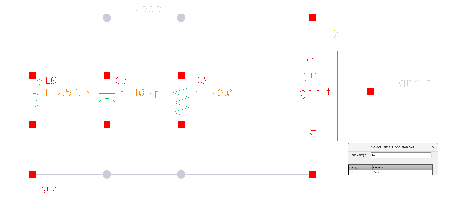
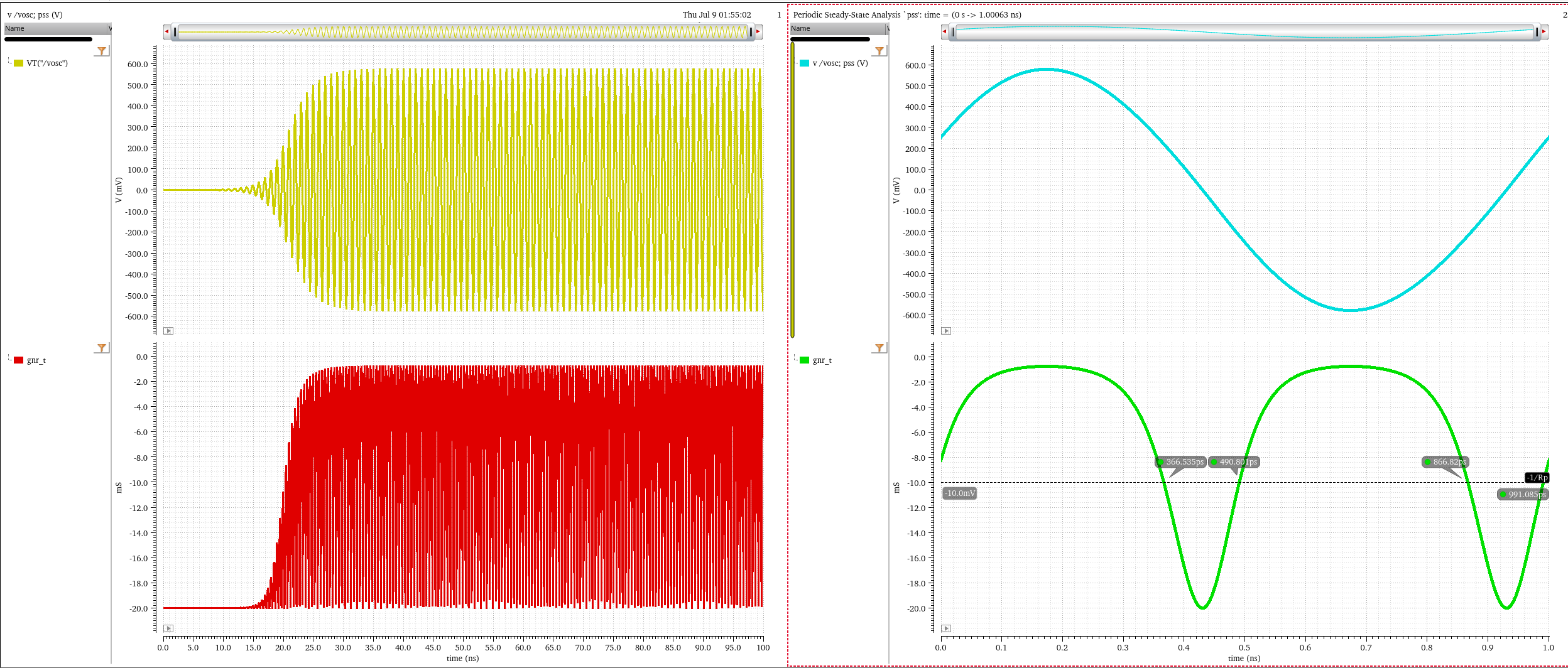
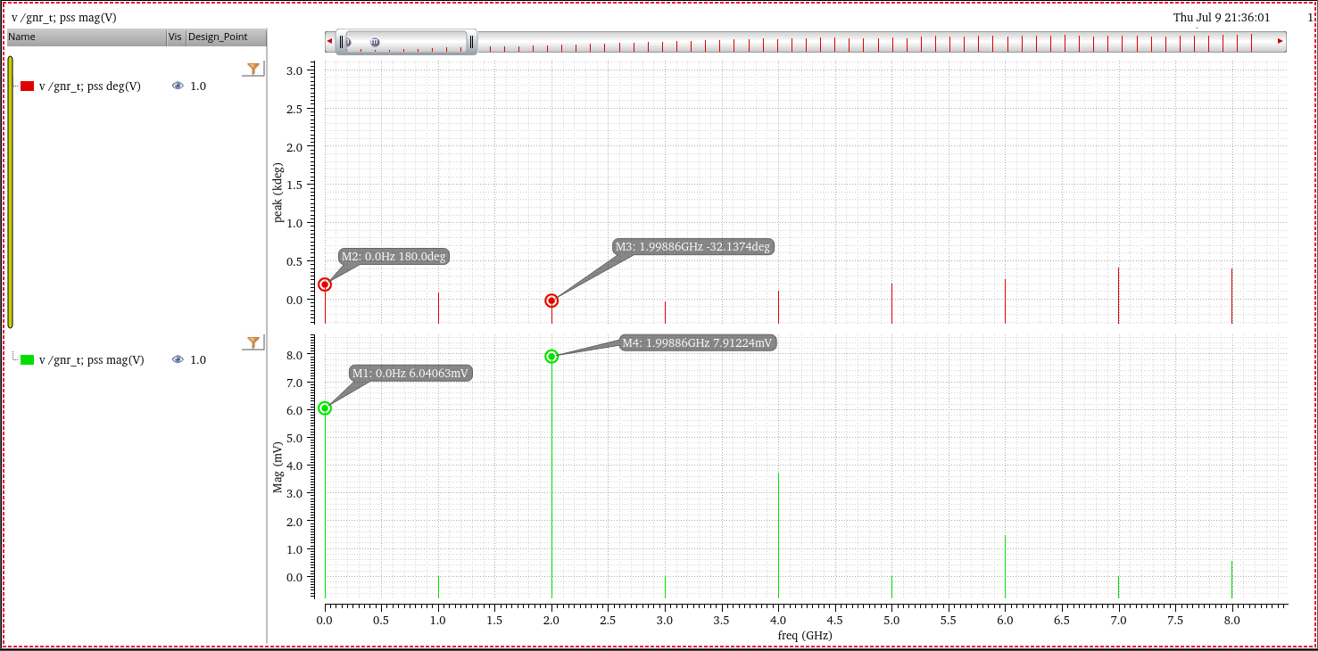
For a symmetric signal \(g_\text{nr}(t)\), the phase angle \(\theta\) is absorbed into the phase shift, transforming the second-harmonic component as: \[ h_{2}(t)=\mathcal{Re}\{2Ae^{j(2\omega _{0}t+\theta )}\}\rightarrow h_{2}(t)=2A\cos (2\omega _{0}t) \]
This yields \(G_\text{nr}[2] = G_\text{nr}[-2] = A = 3.956\). Consequently, the effective gain is evaluated as: \[ G_{\text{eff}}=G_{\text{nr}}[0]-G_{\text{nr}}[2]=-9.9968 \approx -\frac{1}{R_p} \]
Because the magnitude of \(G_\text{nr}[2]\) is comparable to that of \(G_\text{nr}[0]\), \(G_\text{nr}[2]\) must be retained
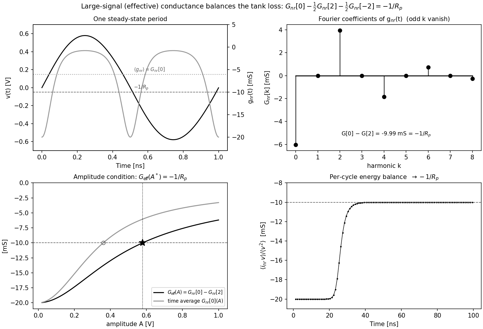
[credits to Claude Fable 5, GPT 5.6 Sol]
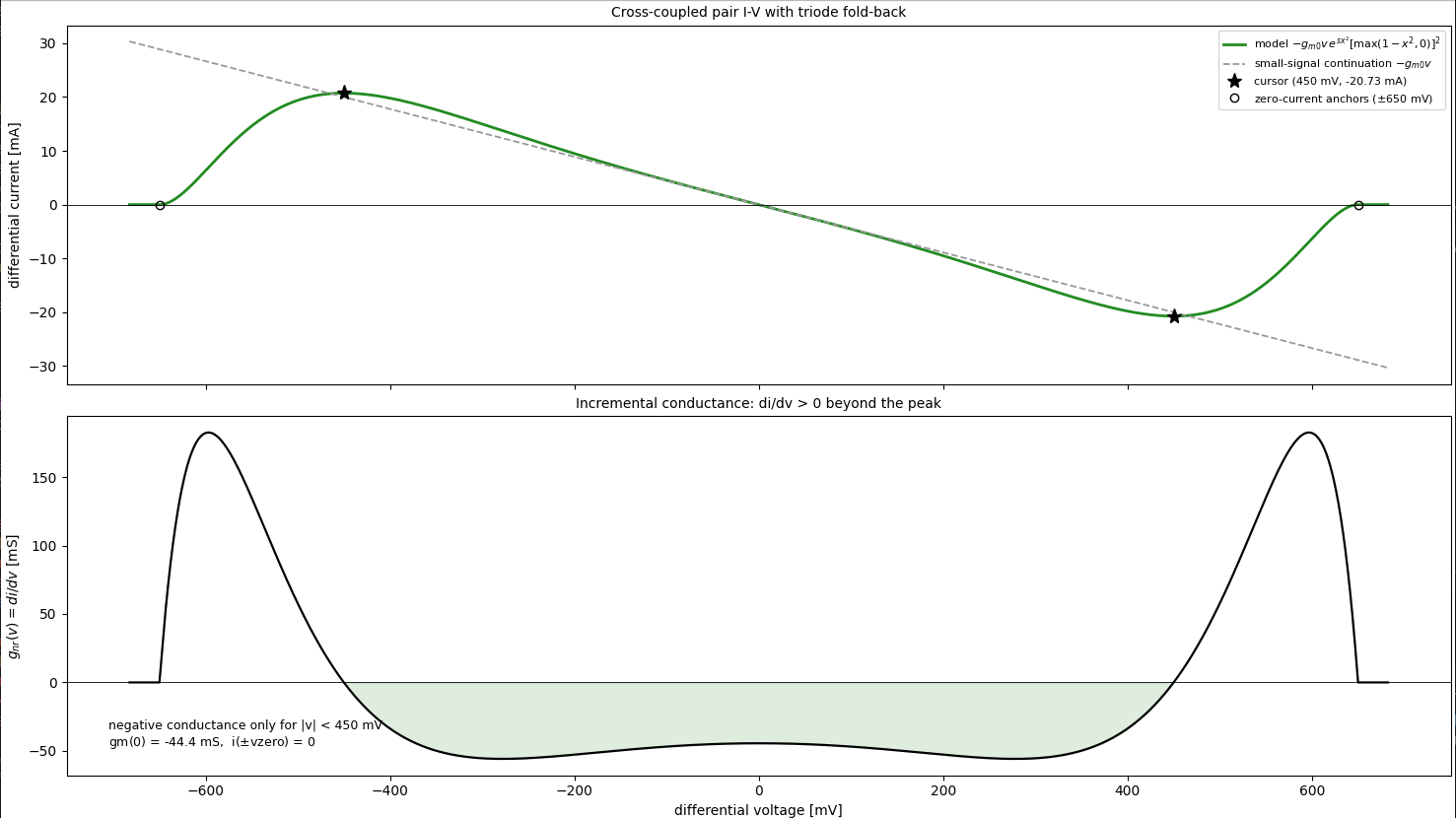
The implemented equation is
\[ i(v)=-g_{m0}v\,e^{s x^2}\left[\max(1-x^2,0)\right]^2, \qquad x=\frac{v}{v_{\mathrm{zero}}} \]
where \(s\) is
shape.
Parameter meanings:
v: differential voltage in volts.gm0: magnitude of the small-signal negative conductance in siemens.vzero: voltage where current reaches zero.shape: dimensionless parameter controlling where the current peak occurs.
At \(v=0\), \(\left.\frac{di}{dv}\right|_{v=0}=-g_{m0}\)
1 | VPK, IPK, VZERO = 0.45, 20.73e-3, 0.65 |
Derivation of \(I_{nr}[k]\) Using Fourier Series and Fourier Transform
Let
\[ v_{nr}(t)=\sum_{l=-\infty}^{\infty}V_{nr}[l]e^{jl\omega_0 t} \]
\[ g_{nr}(t)=\sum_{m=-\infty}^{\infty}G_{nr}[m]e^{jm\omega_0 t} \]
and
\[ i_{nr}(t)=\sum_{k=-\infty}^{\infty}I_{nr}[k]e^{jk\omega_0 t}. \]
The starting equation is
\[ \frac{d i_{nr}(t)}{dt} = g_{nr}(t)\frac{d v_{nr}(t)}{dt}. \]
Method 1: Directly Using Fourier Series
Differentiate \(v_{nr}(t)\):
\[ \frac{d v_{nr}(t)}{dt} = \sum_l jl\omega_0 V_{nr}[l]e^{jl\omega_0 t} \]
Multiply by \(g_{nr}(t)\):
\[ g_{nr}(t)\frac{d v_{nr}(t)}{dt} = \left(\sum_m G_{nr}[m]e^{jm\omega_0 t}\right) \left(\sum_l jl\omega_0 V_{nr}[l]e^{jl\omega_0 t}\right) \]
\[ = \sum_m\sum_l jl\omega_0 V_{nr}[l]G_{nr}[m] e^{j(l+m)\omega_0 t} \]
For the \(k\)-th harmonic,
\[ l+m=k \]
so
\[ m=k-l. \]
Therefore,
\[ \left[g_{nr}(t)\frac{d v_{nr}(t)}{dt}\right]_k = \sum_l jl\omega_0 V_{nr}[l]G_{nr}[k-l] \]
But
\[ \frac{d i_{nr}(t)}{dt} = \sum_k jk\omega_0 I_{nr}[k]e^{jk\omega_0 t} \]
so the \(k\)-th coefficient is
\[ jk\omega_0 I_{nr}[k]. \]
Therefore, for \(k\neq 0\),
\[ jk\omega_0 I_{nr}[k] = \sum_l jl\omega_0 V_{nr}[l]G_{nr}[k-l] \]
so
\[ \boxed{ I_{nr}[k] = \sum_{l=-\infty}^{\infty} \frac{l}{k} V_{nr}[l]G_{nr}[k-l], \qquad k\neq 0 } \]
The \(l/k\) comes from
\[ \frac{jl\omega_0}{jk\omega_0} = \frac{l}{k}. \]
Method 2: Indirectly Using Fourier Transform
Use the continuous-time Fourier transform of a periodic signal:
\[ x(t)=\sum_k X[k]e^{jk\omega_0 t} \]
has Fourier transform
\[ X(\omega)=2\pi\sum_k X[k]\delta(\omega-k\omega_0). \]
So
\[ V_{nr}(\omega) = 2\pi\sum_l V_{nr}[l]\delta(\omega-l\omega_0) \]
and
\[ G_{nr}(\omega) = 2\pi\sum_m G_{nr}[m]\delta(\omega-m\omega_0). \]
Now,
\[ \frac{d v_{nr}(t)}{dt} \quad \Longleftrightarrow \quad j\omega V_{nr}(\omega). \]
Therefore,
\[ j\omega V_{nr}(\omega) = 2\pi\sum_l jl\omega_0 V_{nr}[l]\delta(\omega-l\omega_0). \]
Since
\[ \frac{d i_{nr}(t)}{dt} = g_{nr}(t)\frac{d v_{nr}(t)}{dt}, \]
multiplication in time becomes convolution in frequency:
\[ \mathcal{F}\left\{ g_{nr}(t)\frac{d v_{nr}(t)}{dt} \right\} = \frac{1}{2\pi} G_{nr}(\omega)* \left(j\omega V_{nr}(\omega)\right). \]
Substitute the impulse-train spectra:
\[ = \frac{1}{2\pi} \left( 2\pi\sum_m G_{nr}[m]\delta(\omega-m\omega_0) \right) * \left( 2\pi\sum_l jl\omega_0 V_{nr}[l]\delta(\omega-l\omega_0) \right) \]
\[ = 2\pi \sum_m\sum_l jl\omega_0 G_{nr}[m]V_{nr}[l] \delta(\omega-(m+l)\omega_0). \]
For the \(k\)-th harmonic,
\[ m+l=k \]
so
\[ m=k-l. \]
Thus,
\[ \mathcal{F}\left\{ g_{nr}(t)\frac{d v_{nr}(t)}{dt} \right\} = 2\pi \sum_k \left[ \sum_l jl\omega_0 V_{nr}[l]G_{nr}[k-l] \right] \delta(\omega-k\omega_0). \]
But
\[ \frac{d i_{nr}(t)}{dt} \quad \Longleftrightarrow \quad j\omega I_{nr}(\omega). \]
Since
\[ I_{nr}(\omega) = 2\pi\sum_k I_{nr}[k]\delta(\omega-k\omega_0), \]
we get
\[ j\omega I_{nr}(\omega) = 2\pi\sum_k jk\omega_0 I_{nr}[k]\delta(\omega-k\omega_0). \]
Equating the \(k\)-th impulse coefficient:
\[ jk\omega_0 I_{nr}[k] = \sum_l jl\omega_0 V_{nr}[l]G_{nr}[k-l]. \]
Therefore,
\[ \boxed{ I_{nr}[k] = \sum_l \frac{l}{k} V_{nr}[l]G_{nr}[k-l], \qquad k\neq 0 } \]
Frequency Modulation Effects
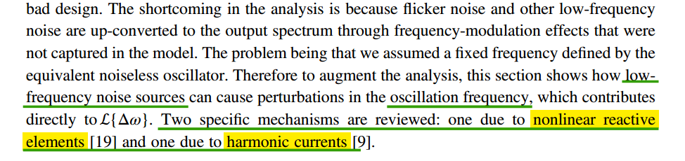
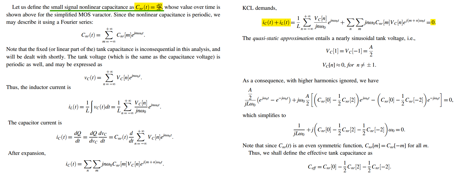
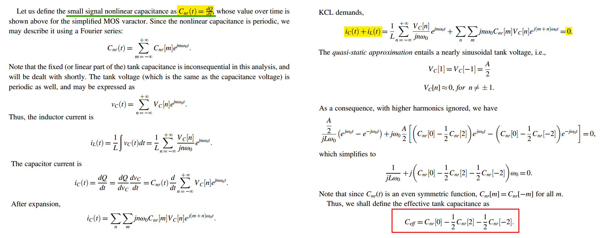
Ceff - large signal capacitance
E. Hegazi and A. A. Abidi, "Varactor characteristics, oscillator tuning curves, and AM-FM conversion," in IEEE Journal of Solid-State Circuits, vol. 38, no. 6, pp. 1033-1039, June 2003 [https://sci-hub.jp/10.1109/JSSC.2003.811968]
TODO 📅
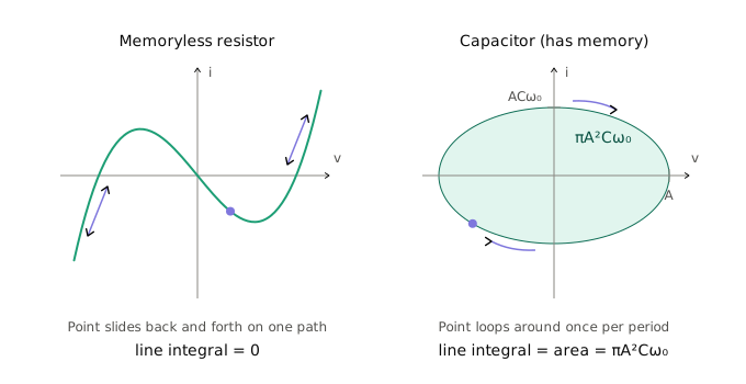
\[ \boxed{\oint i_{nr}\,dv_{nr} = \int_0^T i_{nr}(t)\frac{dv_{nr}(t)}{dt}\,dt} \] It is the signed area-related quantity swept in the \(i\)-\(v\) plane over one period, which is used as a memory detector — a one-line mathematical test for whether an element's behavior depends on its history
Groszkowski's Effect
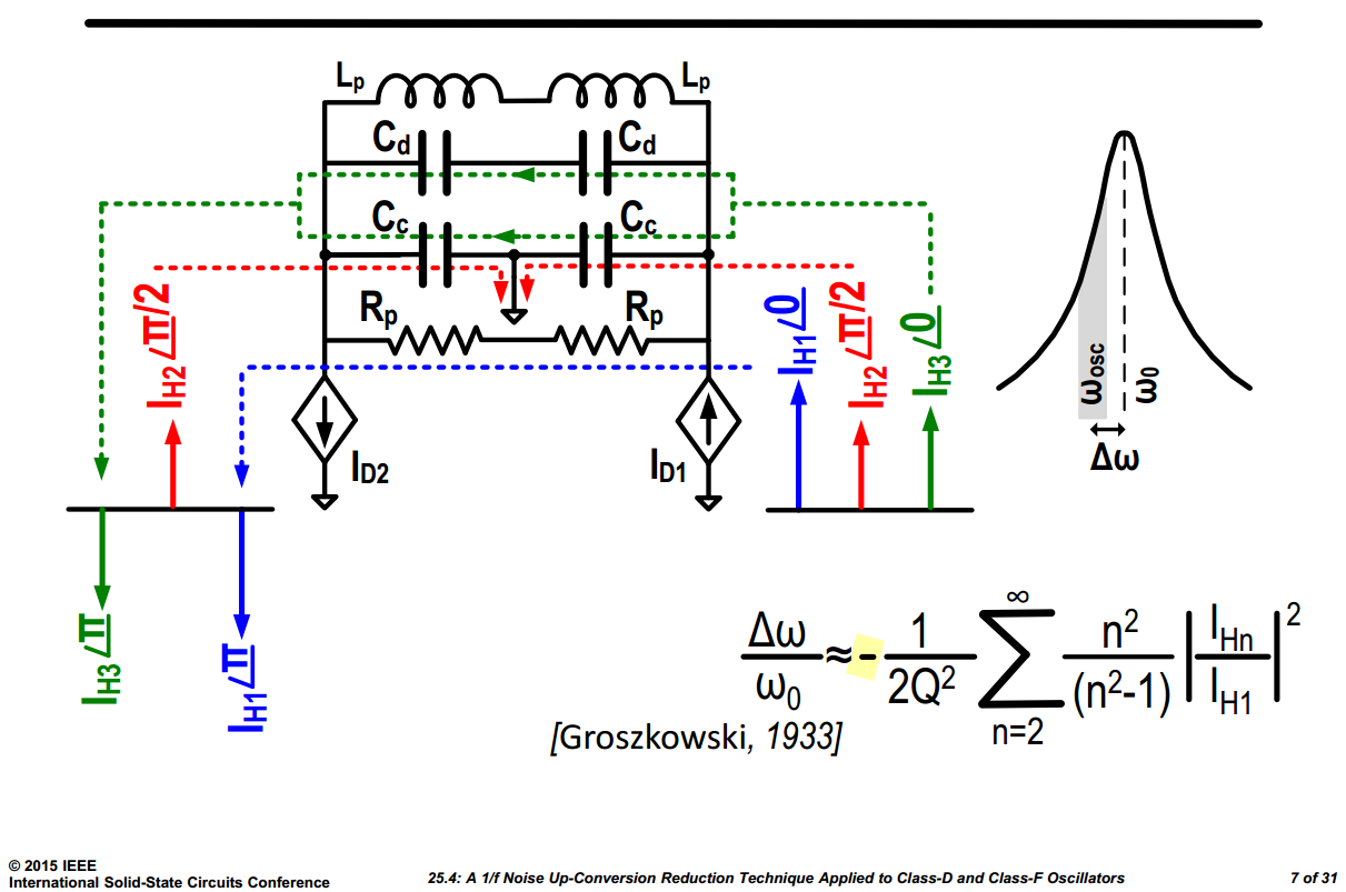
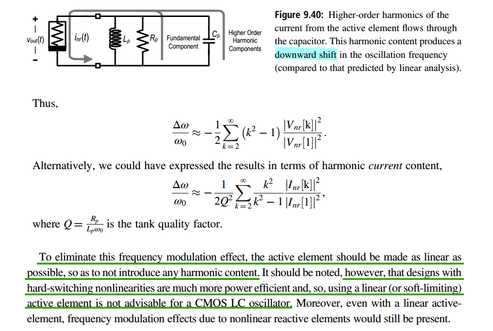
indirect injection of flicker noise from the tail current source was analyzed by "Groszkowski effect" (different from the ISF theory). However it fails to explain the \(1/f\) noise upconversion from the cross-coupled pair
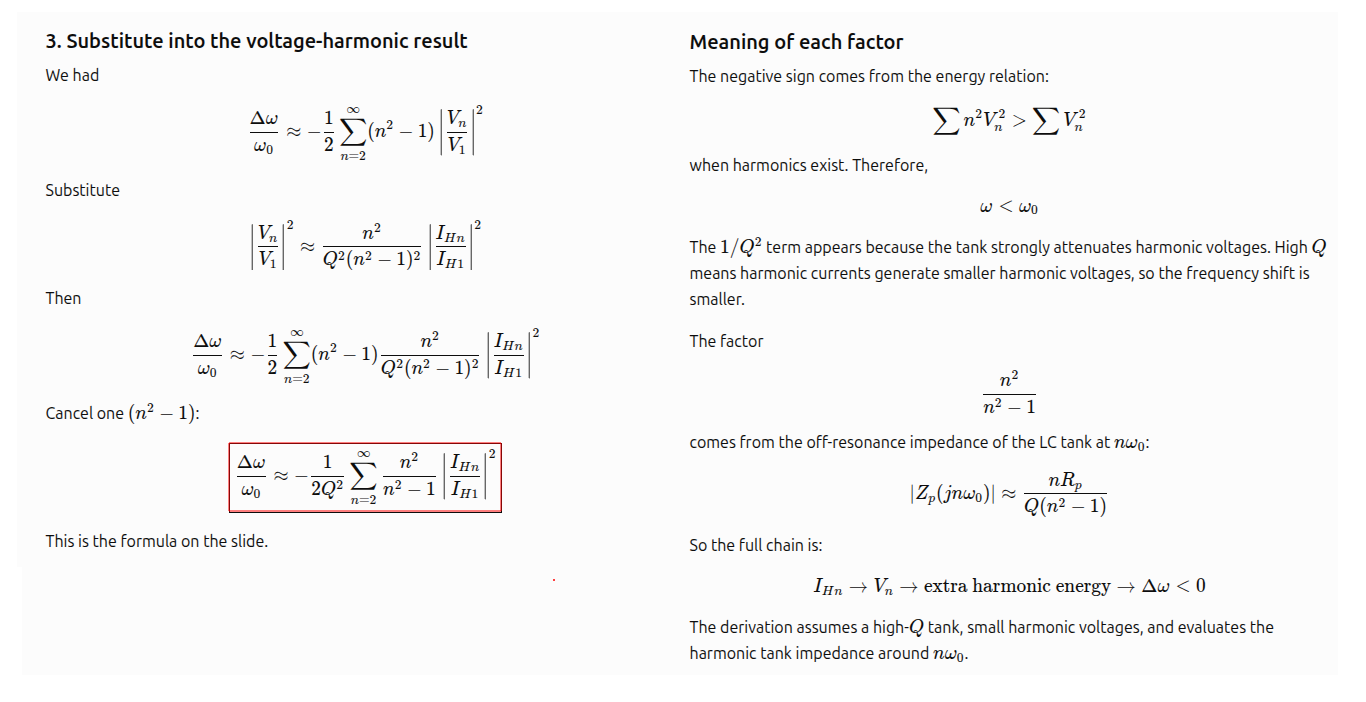
The Groszkowski effect relies on AM-to-FM conversion: nonlinearities make the oscillation frequency amplitude-dependent, so amplitude fluctuations are converted into frequency fluctuation
\[ \delta \omega = \frac{\partial \omega_0}{\partial A}\, \delta A. \]
Thus, the flicker noise from the tail current source is converted into phase noise through the following sequence:
\[ \text{Tail }1/f\ \text{noise} \;\rightarrow\; \text{amplitude fluctuation} \;\rightarrow\; \text{frequency shift} \;\rightarrow\; \text{phase noise} \]
The oscillator phase is perturbed directly for the cross-coupled pair
\[ \text{Cross-coupled }1/f\ \text{noise} \;\rightarrow\; \text{direct timing error} \;\rightarrow\; \text{phase noise}. \]
Unlike the Groszkowski effect, this mechanism does not rely on amplitude-to-frequency conversion
credits to GPT-5.5 High
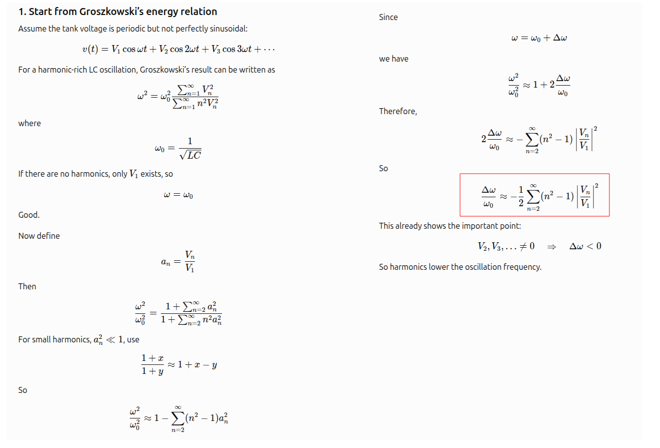
Groszkowski's effect is an oscillator frequency shift caused by harmonic content in the oscillation waveform/current
For a periodic LC oscillation, the average stored energy must balance between \(C\) and \(L\)
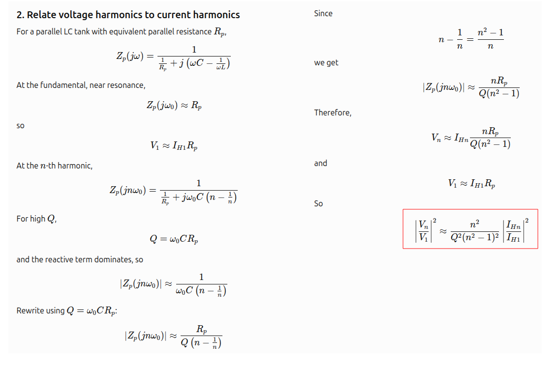
average energy balance \(\overline{W_L}=\overline{W_C}\), or equivalently \[ \sum L I_n^2 = \sum C V_n^2 \] \(I_n\) here is the reactive tank current harmonic, not directly the transistor current harmonic \(I_{Hn}\) in the slide
On-Chip Inductors and Transformer
hai-kun, 片上电感的版图优化方法 [https://zhuanlan.zhihu.com/p/37479700]
—, 电磁场仿真与片上电感的优化讲座实录 [https://zhuanlan.zhihu.com/p/37942671]
—, 片上变压器的应用与设计 (二)多峰值谐振腔 [https://zhuanlan.zhihu.com/p/45799676]
Sunderarajan S. Mohan, Modeling, Design and Optimization of On-Chip Inductors and Transformers [http://www-smirc.stanford.edu/papers/Orals99s-mohan.pdf]
W. Leng and A. A. Abidi, "Approximate Equivalent Circuits to Understand Tradeoffs in Geometry of On-Chip Inductors," in IEEE Transactions on Circuits and Systems I: Regular Papers, vol. 68, no. 3, pp. 975-988, March 2021 [https://sci-hub.ru/10.1109/TCSI.2020.3047987]
8-shaped inductor
NXP BV, US8183971B2, 8-shaped inductor [pdf]
Marvell, US9077310B2, Pseudo-8-shaped inductor [pdf]
P. Guan et al., "8-Shaped Inductors: An Essential Addition to RFIC Designers' Toolbox," in IEEE Open Journal of the Solid-State Circuits Society, vol. 4, pp. 131-146, 2024 [pdf]
M. Pisati et al., "A 243-mW 1.25–56-Gb/s Continuous Range PAM-4 42.5-dB IL ADC/DAC-Based Transceiver in 7-nm FinFET," in IEEE Journal of Solid-State Circuits, vol. 55, no. 1, pp. 6-18, Jan. 2020 [https://sci-hub.ru/10.1109/JSSC.2019.2936307]
An 8-shaped (figure-8) inductor is a specialized on-chip, high-Q component used to mitigate electromagnetic coupling and reduce frequency pulling in VCOs by generating opposing, self-canceling magnetic fields
TODO 📅
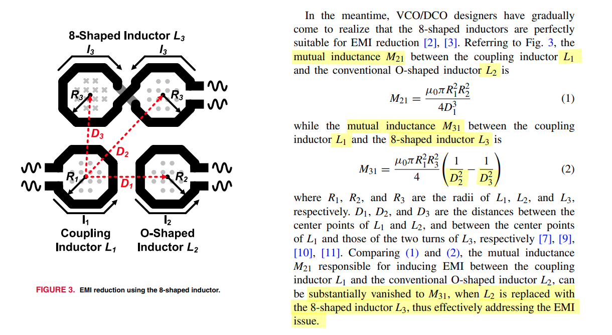
Zou, Wei & Zou, Xuecheng & Ren, Daming & Zhang, Kefeng & Liu, Dongsheng & Ren, Zhixiong. (2019). 2.49-4.91 GHz wideband VCO with optimised 8-shaped inductor. Electronics Letters. [https://sci-hub.jp/10.1049/el.2018.6012]
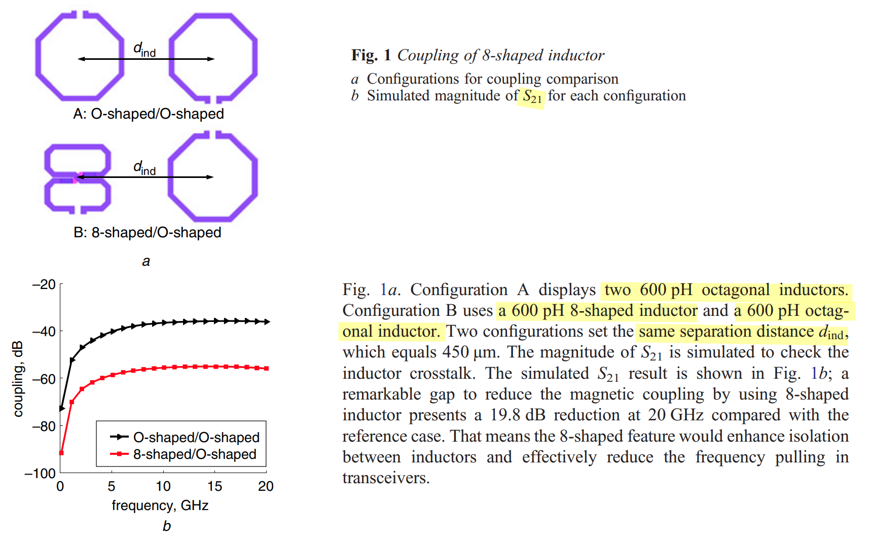
Transformer
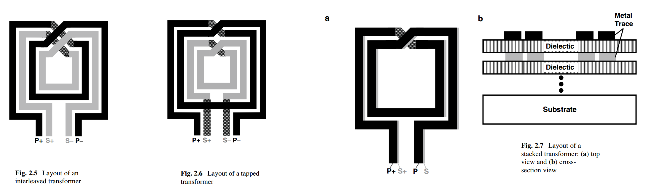
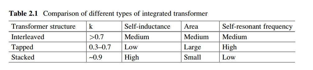
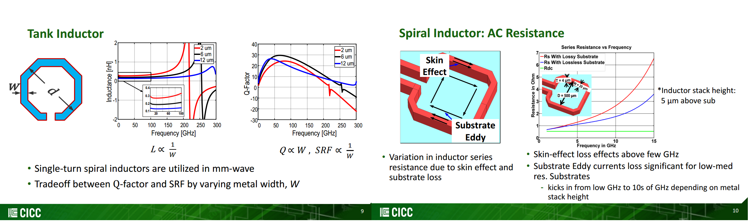
single-turn spiral
To Achieve Low PN
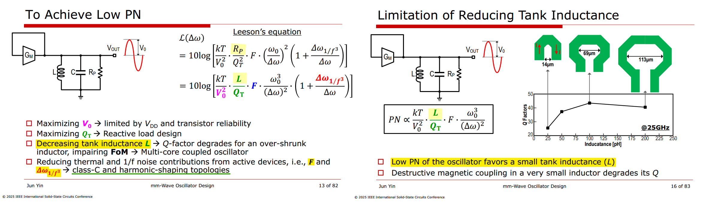
For example, halving \(L\) while holding frequency, \(Q_T\), and \(F\) fixed gives:
| Constraint | Result |
|---|---|
| Constant voltage amplitude | Phase noise improves by 3 dB; required current and tank power double |
| Constant drive current, current limited | Amplitude halves; phase noise worsens by 3 dB |
| Constant tank dissipation i.e. \(V_0^2/R_p=\mathrm{constant}\) | Amplitude falls by \(1/\sqrt2\); phase noise stays unchanged |
On-Chip Capacitor
A. Bonfanti, S. Levantino, C. Samori and A. L. Lacaita, "A varactor configuration minimizing the amplitude-to-phase noise conversion in VCOs," in IEEE Transactions on Circuits and Systems I: Regular Papers, vol. 53, no. 3, pp. 481-488, March 2006 [https://sci-hub.ru/10.1109/TCSI.2005.858764]
monolithic C-V characteristic
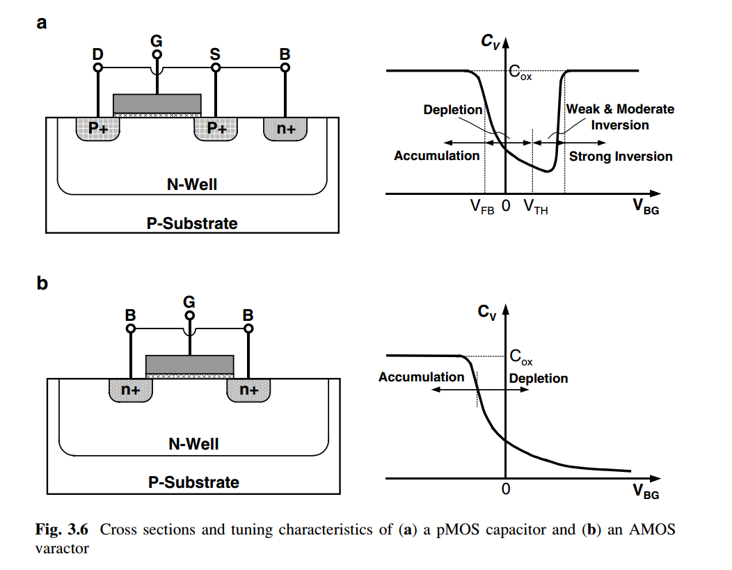
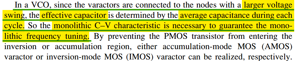
MOS varactor
characterized by by quality factor and capacitance ratio factor
tuning range

VCO gain \(K_{\mathrm{VCO},f}\) in \(\text{Hz}/V\) \[ \boxed{K_{\mathrm{VCO},f}=\frac{df_0}{dV}=-\frac{f_0}{2C}K_v} \]
where \(K_v\) is the varactor capacitance sensitivity (\(F/V\))
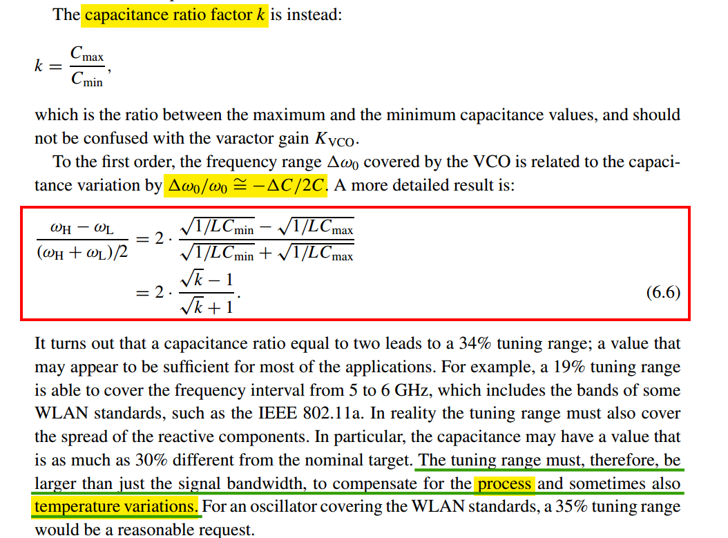
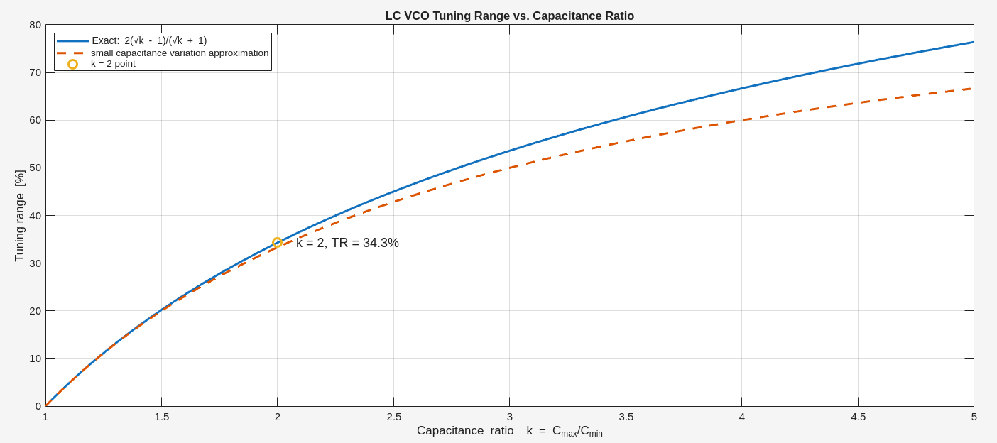
\[ \Delta\omega_0 = \frac{\partial \omega_0}{\partial C}\cdot \Delta C = -\frac{\Delta C}{2C}\cdot \omega_0 \] For tuning range, use the magnitude: \[ TR_{\text{approx}} \approx \frac{1}{2}\frac{C_{\max}-C_{\min}}{C_{\text{avg}}} \] where \(C_{\text{avg}}=\frac{C_{\max}+C_{\min}}{2}\)
Therefore: \[ TR_{\text{approx}} \approx \frac{1}{2} \frac{C_{\max}-C_{\min}} {(C_{\max}+C_{\min})/2} \] Now divide numerator and denominator by \(C_{\min}\): \[ TR_{\text{approx}} = \frac{C_{\max}/C_{\min}-1} {C_{\max}/C_{\min}+1} \] Since \(k=\frac{C_{\max}}{C_{\min}}\)
we get \[ \boxed{ TR_{\text{approx}} = \frac{k-1}{k+1} } \]
capacitance ratio factor
quality factor
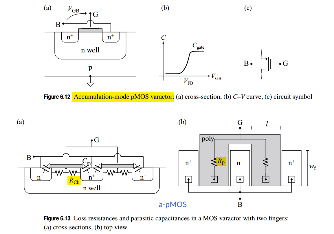
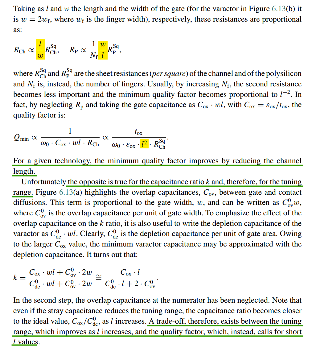
Two resistances, both in series with the variable capacitance:
- RCh is the channel resistance of the accumulation layer
- RP is the gate resistance due to the finite polysilicon conductivity
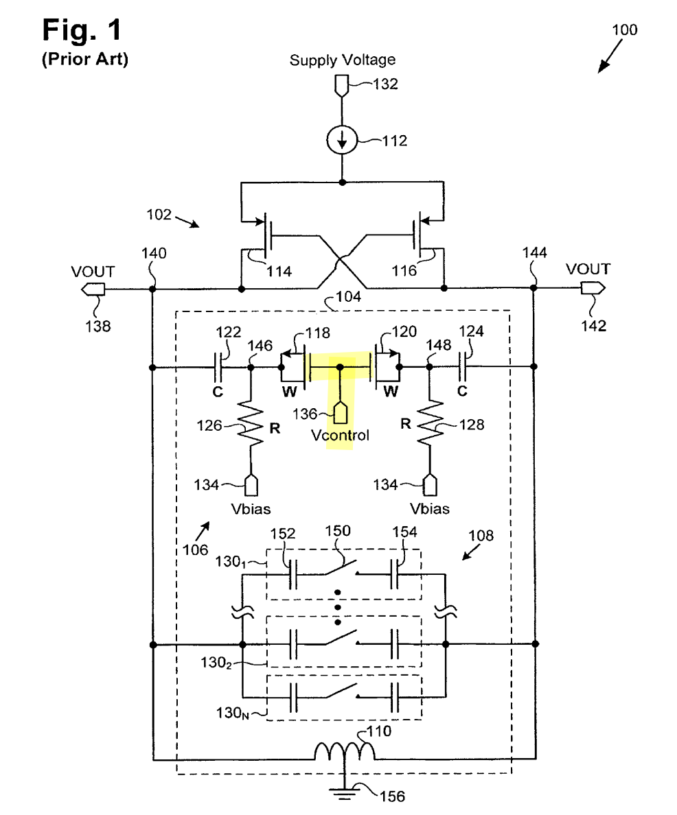
Li, Qiang, et al. Differential varactor circuit for a voltage controlled oscillator. Patent No. US 8,098,109 B2, 17 Jan. 2012 [https://patentimages.storage.googleapis.com/57/d5/16/75bc7e21f7321c/US8098109.pdf]
The VCO varactor introduces a loading effect on the preceding CP-PLL loop filter \[ \color{blue}\boxed{ \text{The VCO varactor is part of the CP-PLL loop-filter load.} } \]
Varactor Tuning Sensitivity

Given
\[ C_{\text{tot}} = C_{mp} + (C_v+C_p)\parallel C_m \]
where \(C_{mp}\), \(C_p\), and \(C_m\) are fixed, while \(C_v=C_v(V)\).
Then
\[ C_{\text{tot}} = C_{mp} + \frac{C_m(C_v+C_p)} {C_m+C_v+C_p}. \]
Using the chain rule,
\[ \frac{dC_{\text{tot}}}{dV} = \frac{\partial C_{\text{tot}}}{\partial C_v} \frac{dC_v}{dV}. \]
Since
\[ \frac{\partial C_{\text{tot}}}{\partial C_v} = \frac{C_m^2} {(C_m+C_v+C_p)^2}, \]
we obtain
\[ \boxed{ \frac{dC_{\text{tot}}}{dV} = \left( \frac{C_m} {C_m+C_v+C_p} \right)^2 \frac{dC_v}{dV} } \]
Therefore, the effective tuning sensitivity \(dC_{\text{tot}}/dV\) is attenuated relative to the intrinsic varactor sensitivity \(dC_v/dV\) by
\[ \left( \frac{C_m} {C_m+C_v+C_p} \right)^2 \]
Capacitor Bank
B. Sadhu and R. Harjani, "Capacitor bank design for wide tuning range LC VCOs: 850MHz-7.1GHz (157%)," Proceedings of 2010 IEEE International Symposium on Circuits and Systems, Paris, France, 2010 [https://sci-hub.st/10.1109/ISCAS.2010.5537040]
TODO 📅
large value KVCO is not favorable due to noise and possibly spurs at the control voltage
varactor AM-PM PN
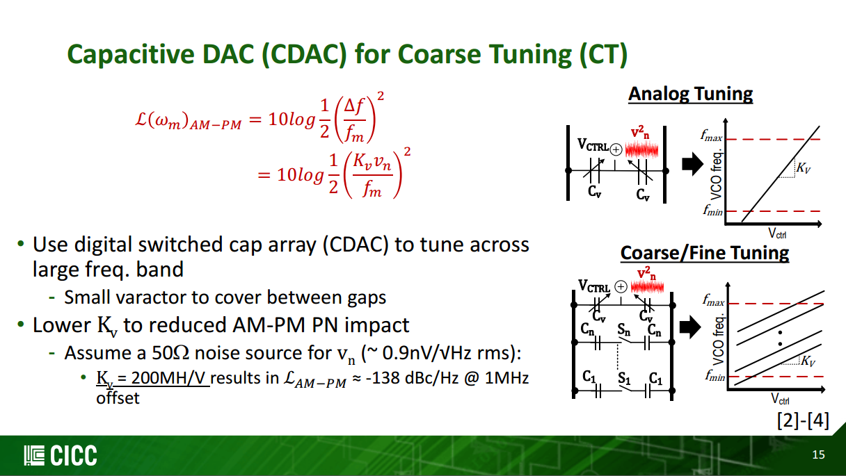
with \(v_n = \sqrt{4kTR} = \sqrt{1.66 \times 10^{-20} \times 50} \approx 0.9 \, \text{nV}/\sqrt{\text{Hz}}\)
1 | octave:1> 10*log10(1/2*(200e6*0.9e-9/1e6)^2) |
FM \(\Delta \omega_0 \cos\omega_m t\) to PM \(\frac{\Delta \omega_0}{\omega_m} \sin\omega_m t\) depend on FM modulation frequency \(\omega_m\) — in frequency domain \(\frac{K_\text{vco} V_n}{s}\)
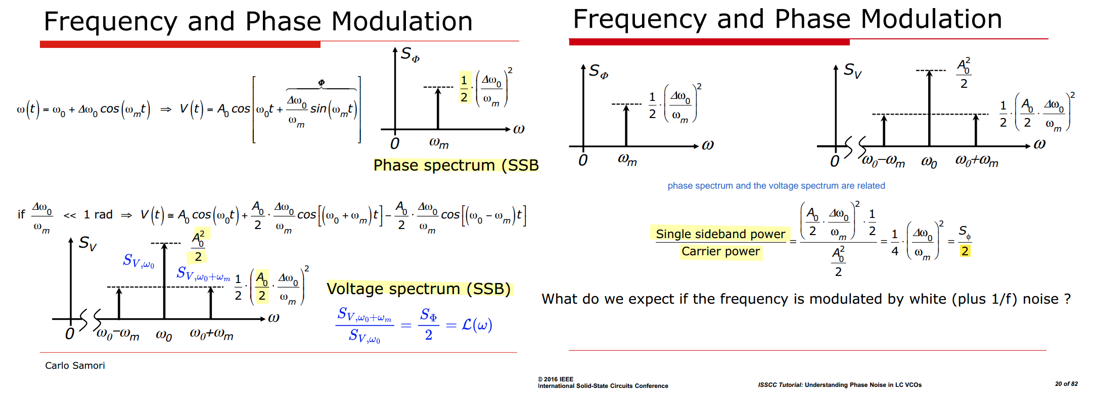

Waleed's CICC slide \(\Delta f = K_\text{v} v_n\) is already an RMS quantity — \(v_n\) is specified as an rms density; Samori's \(\Delta \omega_0\) is the peak deviation of a deterministic sinusoidal test tone.
Connect them with \[ \Delta_{\text{peak}} = \sqrt{2} \cdot \Delta_{\text{rms}} \implies \frac{1}{4} (\sqrt{2} \Delta_{\text{rms}})^2 = \frac{1}{2}\Delta_{\text{rms}}^2 \] Identical physics, different bookkeeping
Tuning Range
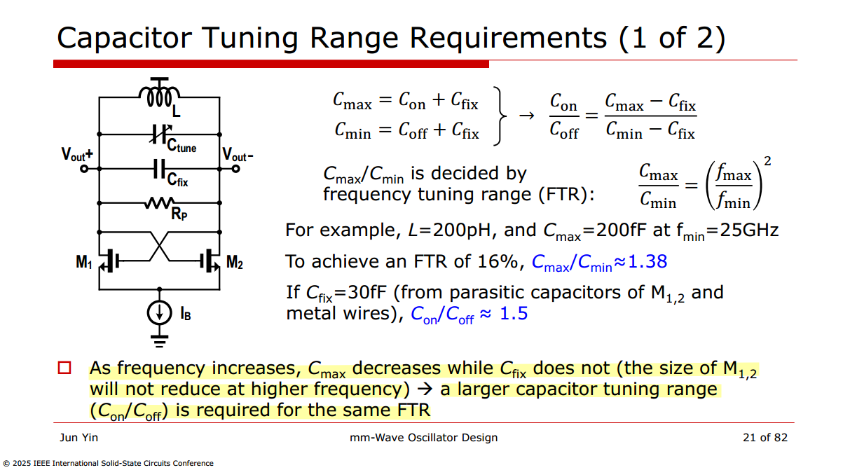 \[
\frac{C_\text{on}}{C_\text{off}} = \frac{C_\text{max} -
C_\text{fix}}{C_\text{min} - C_\text{fix}} =
\frac{C_\text{max}/C_\text{min} -
C_\text{fix}/C_\text{min}}{1-C_\text{fix}/C_\text{min}}
\]
\[
\frac{C_\text{on}}{C_\text{off}} = \frac{C_\text{max} -
C_\text{fix}}{C_\text{min} - C_\text{fix}} =
\frac{C_\text{max}/C_\text{min} -
C_\text{fix}/C_\text{min}}{1-C_\text{fix}/C_\text{min}}
\]
with \(C_\text{max}/C_\text{min} \gt 1\) and \(C_\text{fix}/C_\text{min}\lt 1\)
\[ \frac{C_\text{on}}{C_\text{off}} = K_0 + \frac{K_1}{1-C_\text{fix}/C_\text{min}} \]
For same FTR and higher frequency \[ \text{smaller}\space\space C_\text{min} \implies \text{larger} \space\space \frac{C_\text{on}}{C_\text{off}} \]
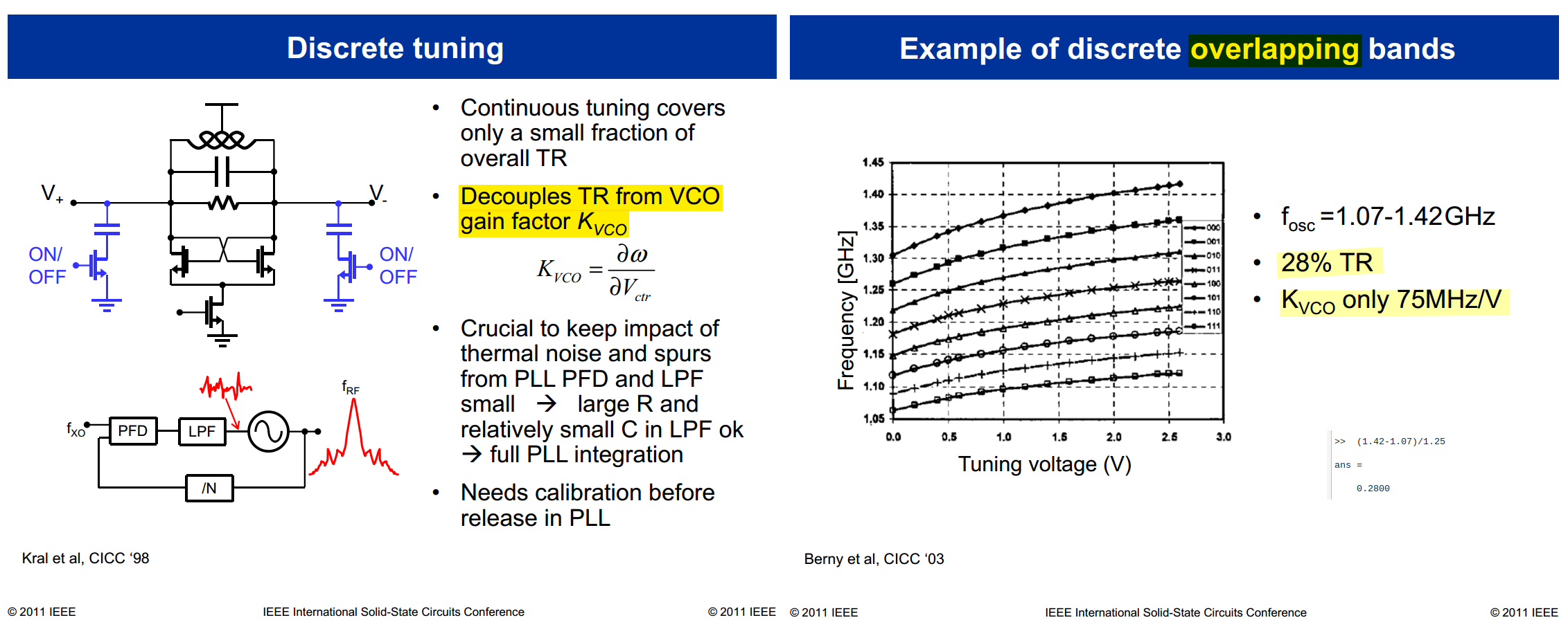
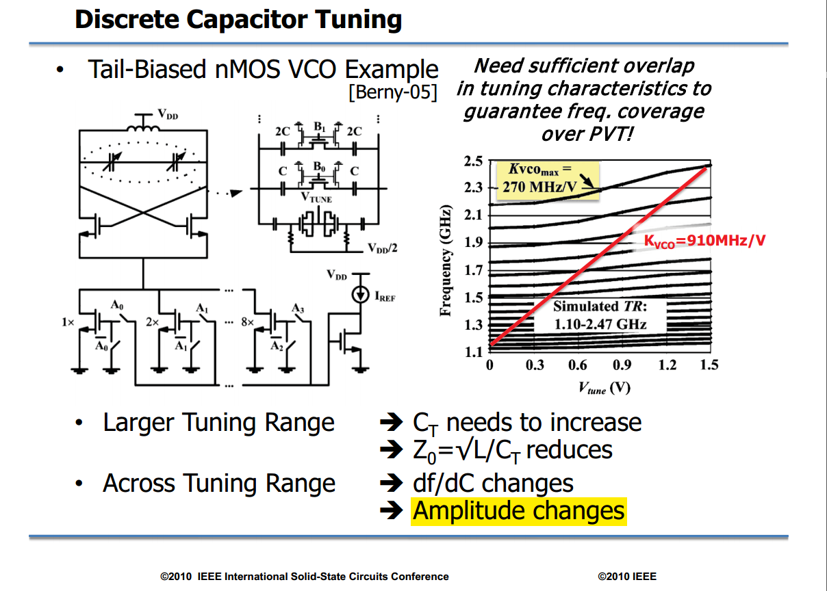
Discrete Capacitor Tuning
A. D. Berny, A. M. Niknejad and R. G. Meyer, "A 1.8-GHz LC VCO with 1.3-GHz tuning range and digital amplitude calibration," in IEEE Journal of Solid-State Circuits, vol. 40, no. 4, pp. 909-917, April 2005 [https://sci-hub.jp/10.1109/JSSC.2004.842851]
D. Turker et al., "A 7.4-to-14GHz PLL with 54fsrms jitter in 16nm FinFET for integrated RF-data-converter SoCs," 2018 IEEE International Solid-State Circuits Conference - (ISSCC), San Francisco, CA, USA, 2018 [https://sci-hub.ru/10.1109/ISSCC.2018.8310342]
Q of SC bank
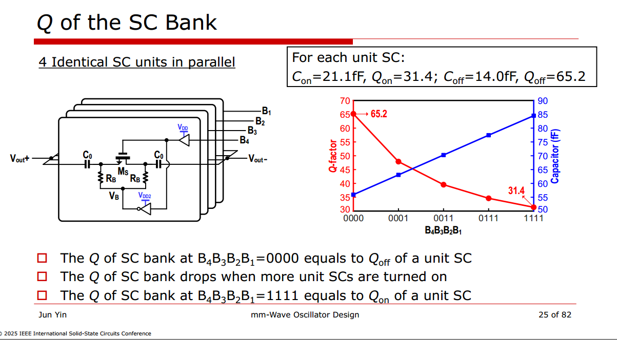
graph LR
    A[Lower f₀] --> B["Larger C_T"]
    B --> C["Lower bank Q"]
    C --> D["Lower tank Q & Lower √(L/C_T)"]
    D --> E["Lower R_p"]
    E --> F["Higher I_bias (for the same amplitude)"]
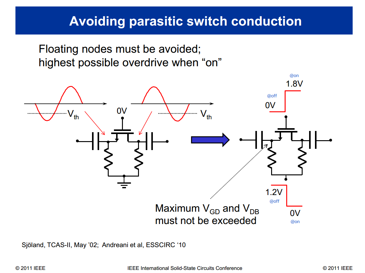
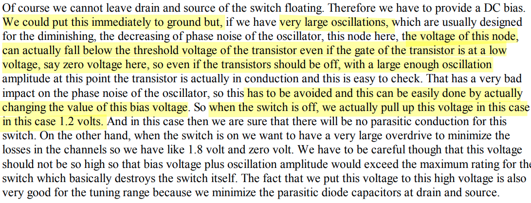
switch resistance effect
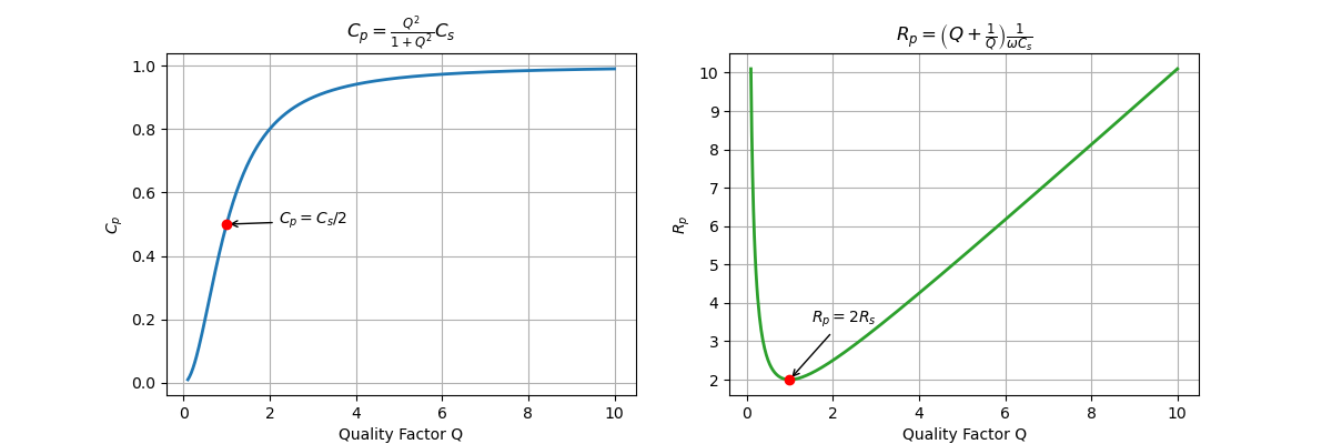
series model (Rs, Cs) to parallel model (Rp, Cp) with fixed Cs but varying Rs
\[ \boxed{C_p = \frac{Q^2}{1+Q^2}C_s=C_s(1-\frac{1}{1+Q^2}) \qquad\qquad R_p = (1+Q^2)R_s = (1+Q^2)\frac{1}{\omega C_s Q}=(\frac{1}{Q}+Q)\frac{1}{\omega C_s}} \]
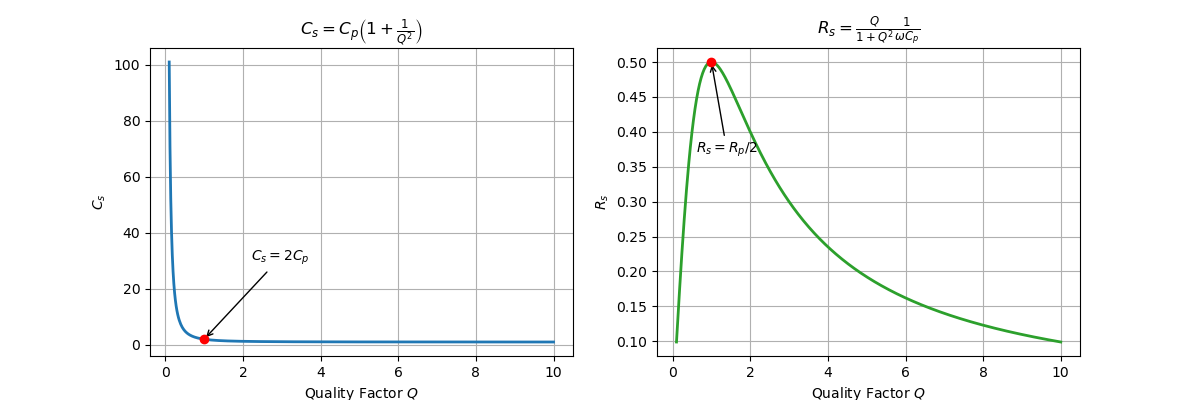
parallel model (Rp, Cp) to series model (Rs, Cs) with fixed Cp but varying Rp \[ \boxed{C_s = \frac{1+Q^2}{Q^2}C_p = C_p(1+\frac{1}{Q^2}) \qquad\qquad R_s = \frac{1}{1+Q^2}R_p = \frac{1}{1+Q^2}\frac{Q}{\omega C_p} = \frac{Q}{1+Q^2}\frac{1}{\omega C_p}} \]
Two Capacitor Q
parallel-combination
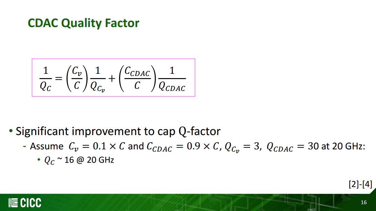
with \(C= C_0 + C_1\) and \(R=\frac{R_0R_1}{R_0+R_1}=\frac{Q_0Q_1}{\omega(C_0Q_1 + C_1Q_0)}\), the combined \(Q_C\) is \[ Q_C = R\cdot \omega C = \frac{Q_0Q_1}{C_0Q_1+C_1Q_0}C \] therefore \[ \boxed{\frac{1}{Q_C} = \frac{C_0}{C}\frac{1}{Q_0} + \frac{C_1}{C}\frac{1}{Q_1}} \]
series-combination
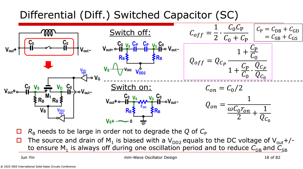
with \(C=\frac{C_0C_1}{C_0+C_1}\), \(R=R_0 + R_1=\frac{1}{\omega}\left(\frac{1}{Q_0C_0}+\frac{1}{Q_1C_1}\right)\) \[ \boxed{Q_C = \frac{1}{\omega R C} = Q_0\frac{1+\frac{C_0}{C_1}}{1+\frac{C_0}{C_1}\frac{Q_0}{Q_1}}} \]
LC Tank Q
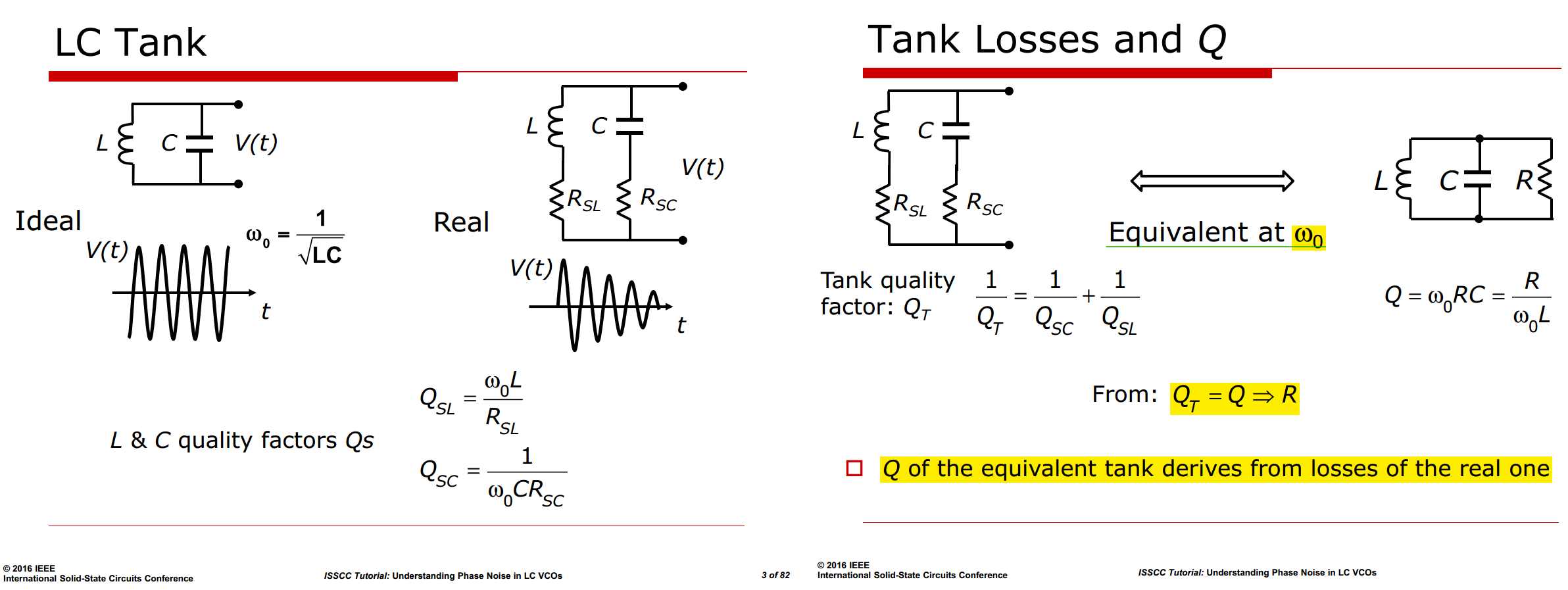
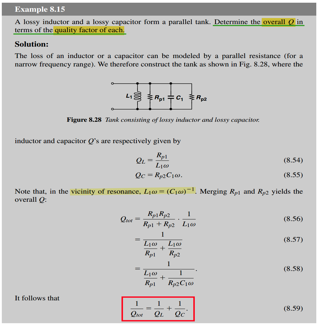
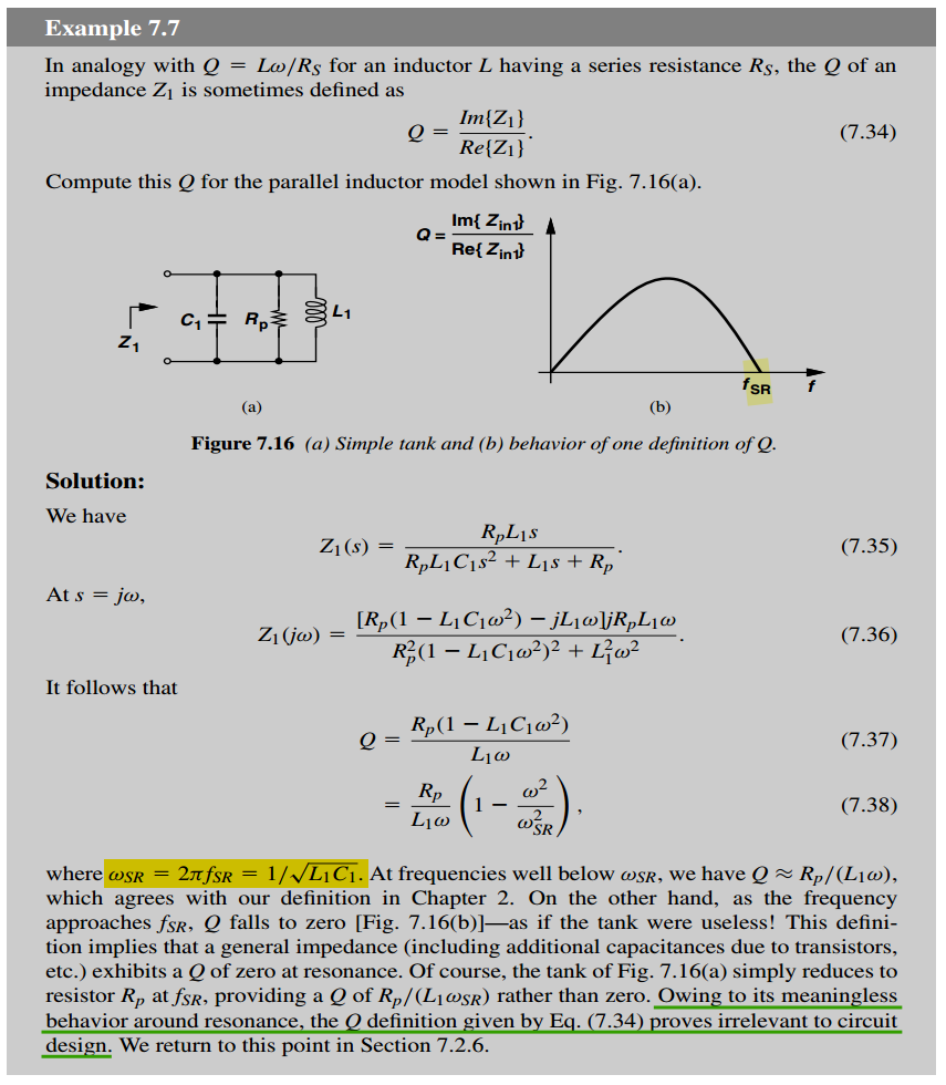
Definitions of Q
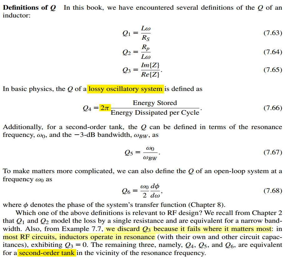
Assuming RLC oscillator waveform is \(V(t)=V_0\sin\omega_0 t\), \(\omega_0 = \frac{1}{\sqrt{LC}}\) is resonant frequency
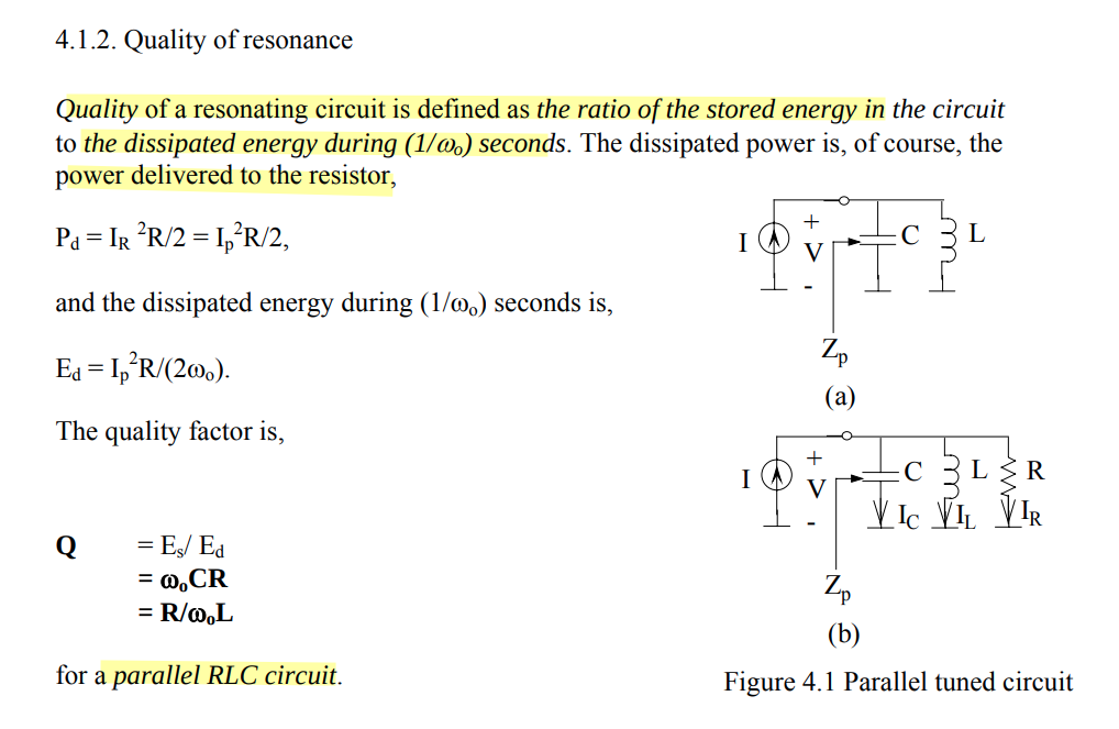
Energy stored \[ E_t = \frac{1}{2}LI_0^2 = \frac{1}{2}CV_0^2 \] Energy Dissipated per Cycle \[ E_d = \frac{V_0^2}{2R}\frac{2\pi}{\omega_0} \] For \(Q_4\), with \(I_0=C\omega_0V_0\) \[ \boxed{Q_4 = 2\pi\frac{E_s}{E_d} = R\omega_0C = \frac{R}{\omega_0L}} \]
which holds at resonance
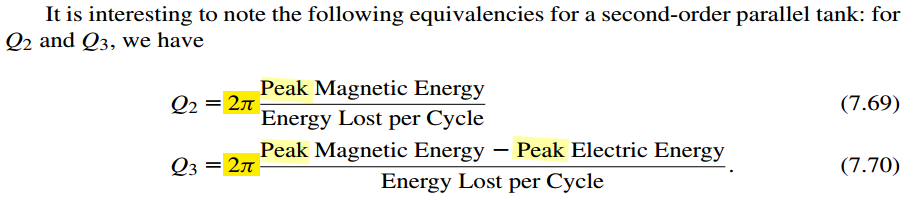
For \(Q_3\), suppose RLC tank is driven by \(V_o\cos \omega t\) voltage source, then
Peak Magnetic Energy \[ E_{pL} = \frac{1}{2}LI_0^2 = \frac{1}{2}L\left(\frac{V_0}{L\omega}\right)^2 \] Peak Electric Energy \[ E_{pC} = \frac{1}{2}CV_0^2 \] with Energy Lost per Cycle \(E_d = \frac{V_0^2}{2R}\frac{2\pi}{\omega_0}\), we have \[ Q_3 = \frac{E_{pL} - E_{pC}}{E_d} = \left(\frac{1}{L\omega^2}-C\right)R\omega=\frac{R}{L\omega}\left(1 - \frac{\omega^2}{\omega^2_{SR}}\right) \]
EEE 211 ANALOG ELECTRONICS [https://www.ee.bilkent.edu.tr/~eee211/LectureNotes/Chapter%20-%2004.pdf]
Tank Impedance Near Resonance
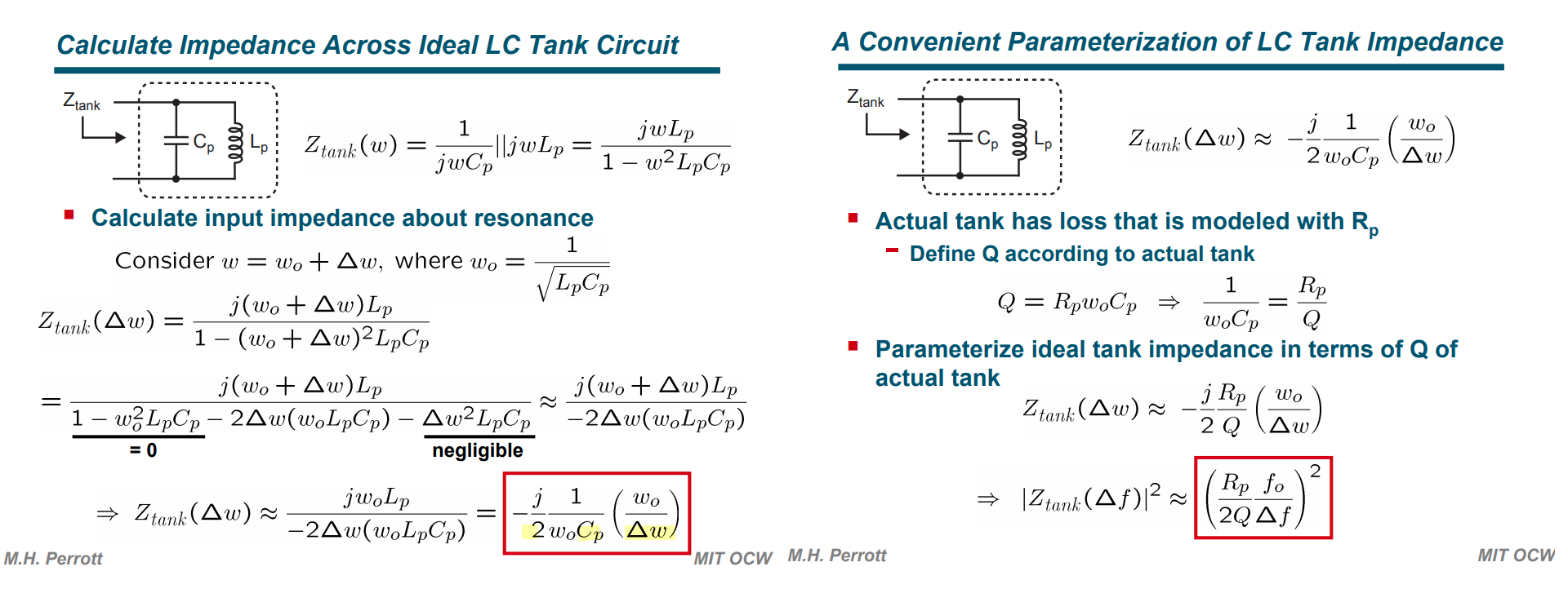 \[
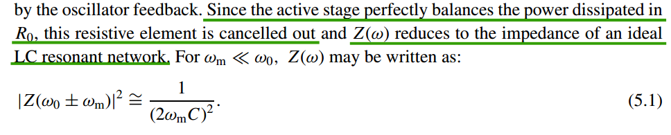
\boxed{|Z(\omega_0\pm \omega_m)|^2 \cong \frac{1}{(2\omega_m
C)^2}}\qquad\qquad \boxed{|Z(\omega_0\pm \omega_m)|^2 \cong
R^2\left(\frac{\omega_0}{2Q\omega_m}\right)^2}
\]
\[
\boxed{|Z(\omega_0\pm \omega_m)|^2 \cong \frac{1}{(2\omega_m
C)^2}}\qquad\qquad \boxed{|Z(\omega_0\pm \omega_m)|^2 \cong
R^2\left(\frac{\omega_0}{2Q\omega_m}\right)^2}
\]
Loaded Q in CMOS fully differential LC oscillator
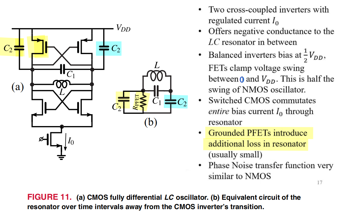

| Regime | \(\omega_0\) | \(Q_{PFET}\) |
|---|---|---|
| Strong PFET, \(R_{PFET} \ll 1/(\omega_0 C_2)\) | \(\dfrac{1}{\sqrt{L(C_1+C_2)}}\) | \(\dfrac{C_1+C_2}{\omega_0 C_2^2 R_{PFET}}\) |
| Weak PFET, \(R_{PFET} \gg 1/(\omega_0 C_2)\) (Eq. 19) | \(\dfrac{1}{\sqrt{L\left(C_1+\frac{C_2}{2}\right)}}\) | \(4\,\omega_0 R_{PFET}\left(C_1+\dfrac{C_2}{2}\right)\) |
Strong PFET, \(R_{PFET} \ll 1/(\omega_0 C_2)\), \(R_{PFET}\) shorts out the left \(C_2\), so the lossy branch is just \(R_{PFET}\) in series with \(C_2\). That series RC branch has its own quality factor
\[ Q_s = \frac{1}{\omega_0 R_{PFET} C_2} \]
The usual series-to-parallel conversion turns it into \(C_2\) in parallel with
\[ R_p = R_{PFET}(1+Q_s^2) \approx \frac{1}{\omega_0^2 C_2^2 R_{PFET}} \]
The tank is now \(L \parallel (C₁ + C₂) \parallel R_p\). Its resonant frequency is \(\omega_0=\dfrac{1}{\sqrt{L(C_1+C_2)}}\), and its \(Q\) is
\[ Q_{PFET} = \omega_0 (C_1+C_2) R_p = \frac{C_1+C_2}{\omega_0 C_2^2 R_{PFET}} = \frac{\sqrt{L(C_1+C_2)}}{C_2 R_{PFET}}\cdot\frac{C_1+C_2}{C_2} \]
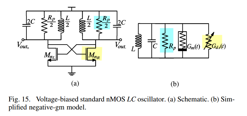
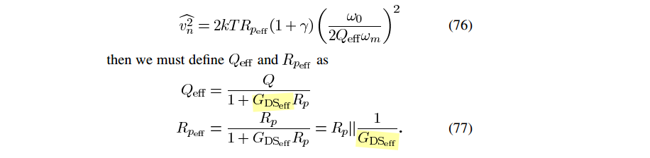
\(G_{ds}\) is parallel with LC tank, thus minimizing \(G_{ds}\) is desirable
XCP Parasitics
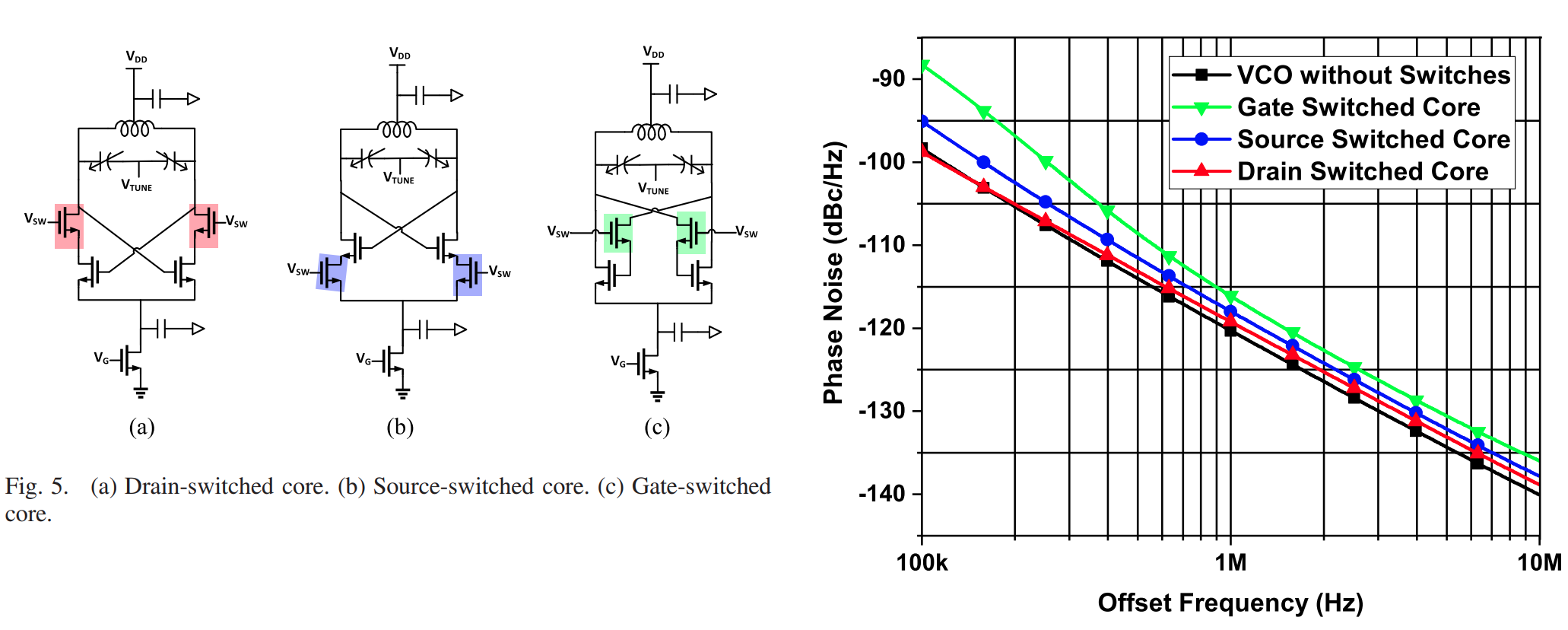
D. Hauspie, E. -C. Park and J. Craninckx, "Wideband VCO With Simultaneous Switching of Frequency Band, Active Core, and Varactor Size," in IEEE Journal of Solid-State Circuits, vol. 42, no. 7, pp. 1472-1480, July 2007 [https://sci-hub.ru/10.1109/JSSC.2007.899105]
Chicco, Francesco, Raffaele Capoccia, Alessandro Pezzotta and Christian C. Enz. “Linear analysis of phase noise in LC oscillators in deep submicron CMOS technologies.” 2017 International Conference on Noise and Fluctuations (ICNF) (2017): 1-4. [https://infoscience.epfl.ch/server/api/core/bitstreams/a022482b-16e8-425f-8a99-3752789a22a9/content]
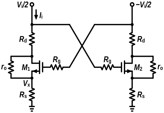
D. Murphy, J. J. Rael and A. A. Abidi, "Phase Noise in LC Oscillators: A Phasor-Based Analysis of a General Result and of Loaded Q," in IEEE Transactions on Circuits and Systems I: Regular Papers, vol. 57, no. 6, pp. 1187-1203, June 2010 [https://sci-hub.ru/10.1109/TCSI.2009.2030110]
Triode on-resistance — Q-degradation
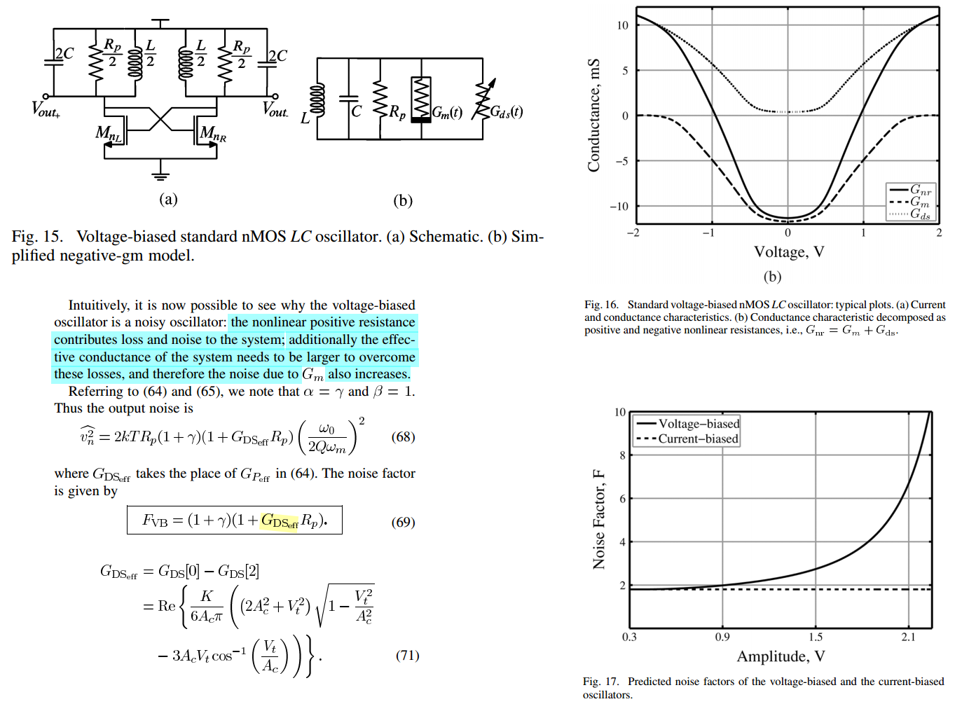
Standard Voltage-Biased nMOS Topology
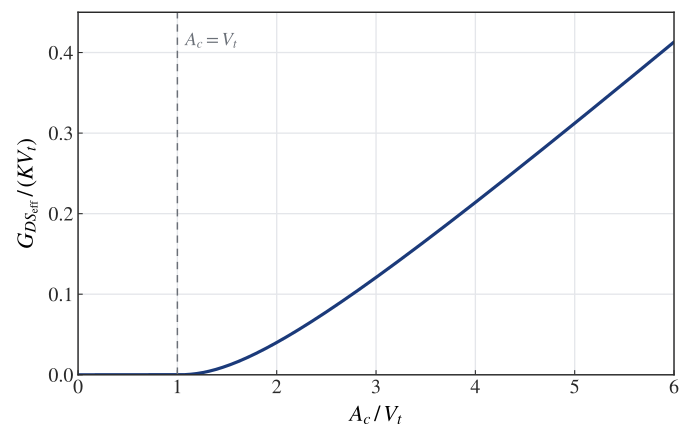
At fixed \(K\) and \(V_t\), \(G_{DS_{\text{eff}}}\) always increases with \(A_c\), so \(F_{VB}\) rises with amplitude
P. Yelleswarapu, A. Jha, R. Willis, Y. Makris and K. K. O, "Phase Noise Reduction in LC VCO’s Using an Array of Cross-Coupled Nanoscale MOSFETs and Intelligent Post-Fabrication Selection," in IEEE Transactions on Microwave Theory and Techniques, vol. 70, no. 6, pp. 3244-3256, June 2022 [https://sci-hub.ru/10.1109/TMTT.2022.3164949]
Pula, Bhanu Teja, Peerla, Rizwan Shaik, Mal, Arindam, Sahoo, Bibhu Datta, Mitigating Gate Resistance in 180 nm CMOS High-Frequency LC-VCOs: Enhanced Performance and Simulation-Model Validation, IET Circuits, Devices & Systems, 2026, 5399291, 11 pages, 2026. https://doi.org/10.1049/cds2/5399291
Gate resistance
The key mechanism is that gate capacitance draws RF current through \(R_g\), creating loss and feedback delay; \(R_g\) also generates thermal voltage noise that modulates the channel current
Seok-Ju Yun, Chong-Yul Cha, Hyoung-Chul Choi and Sang-Gug Lee, "RF CMOSLC-Oscillator With Source Damping Resistors," in IEEE Microwave and Wireless Components Letters, vol. 16, no. 9, pp. 511-513, Sept. 2006 [https://sci-hub.ru/10.1109/LMWC.2006.880700]
A. Hu, D. Liu, Z. Jin, M. Zhang, X. Shan and X. Zou, "A 2.3–5-GHz LC-VCO With Source Damping Resistors to Suppress 1/f Noise Up-Conversion," in IEEE Microwave and Wireless Components Letters, vol. 31, no. 10, pp. 1138-1141, Oct. 2021, doi: 10.1109/LMWC.2021.3107843.
Source resistance
For \(R_s\), remember: \[ Z_{\mathrm{diff}}=-\frac{2}{g_m}-2R_s, \qquad G_{\mathrm{neg}}=-\frac{g_m}{2(1+g_mR_s)} \]
A larger negative-resistance magnitude means weaker loss compensation in a parallel tank.
F. Pepe, A. Bonfanti, S. Levantino, C. Samori and A. L. Lacaita, "Suppression of Flicker Noise Up-Conversion in a 65-nm CMOS VCO in the 3.0-to-3.6 GHz Band," in IEEE Journal of Solid-State Circuits, vol. 48, no. 10, pp. 2375-2389, Oct. 2013 [https://sci-hub.ru/10.1109/JSSC.2013.2273181]
—. Analysis and minimization of flicker noise up-conversion in radio frequency LC-tuned oscillators. 2014. Politecnico di Milano, PhD dissertation [https://www.politesi.polimi.it/bitstream/10589/89783/1/2014_03_PhD_Pepe.pdf]
Drain resistance
layout philosophy
S. Shahramian, "Tutorial: The Art of mm-Wave Design and Layout," 2023 IEEE International Solid-State Circuits Conference (ISSCC), San Francisco, CA, USA, 2023
Patrick Reynaert (KU Leuven), "The Art of CMOS RF Design & Layout" [https://hoomanreyhani.com/product/2025j/]
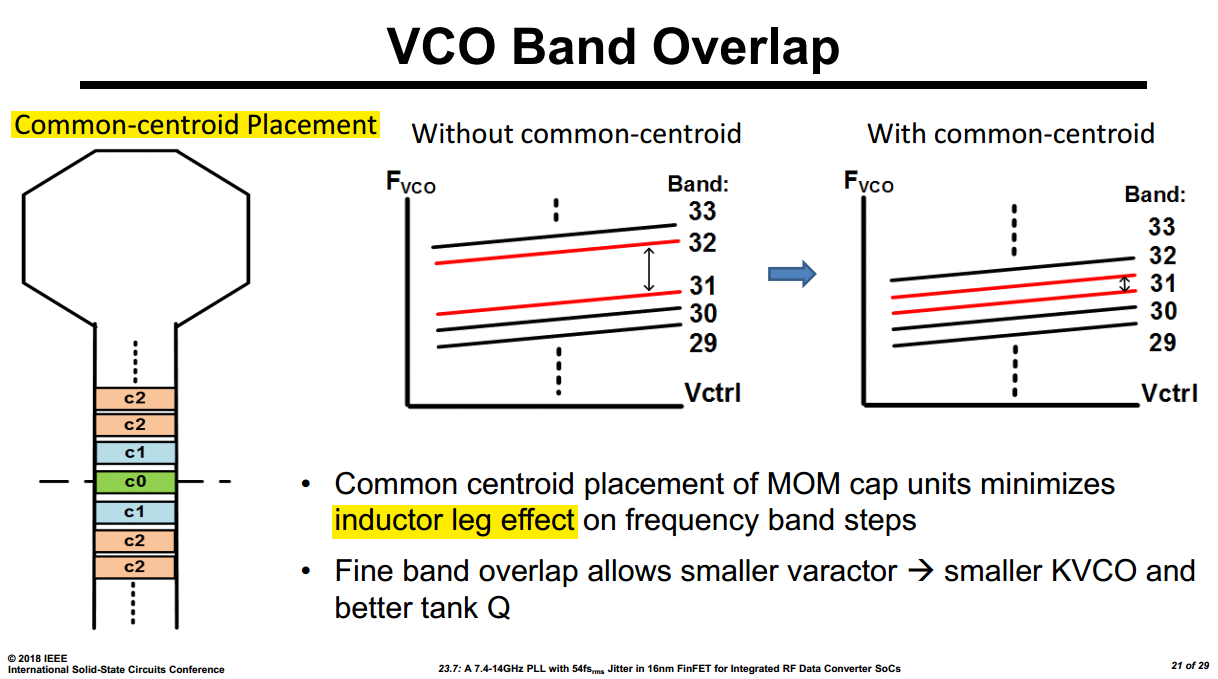
D. Turker et al., "A 7.4-to-14GHz PLL with 54fsrms jitter in 16nm FinFET for integrated RF-data-converter SoCs," 2018 IEEE International Solid-State Circuits Conference - (ISSCC), San Francisco, CA, USA, 2018 [https://sci-hub.ru/10.1109/ISSCC.2018.8310342]
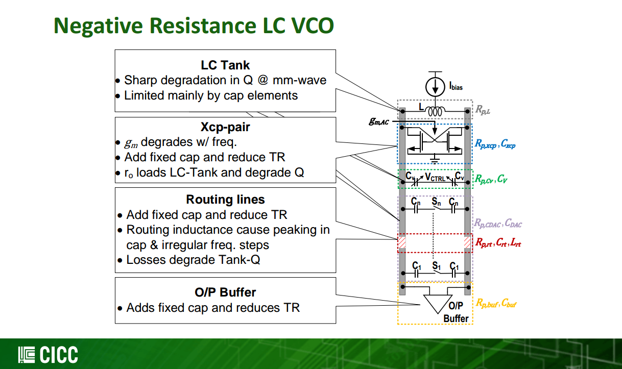
In a differential LC VCO, every tuning bit should preserve the symmetry of the two tank nodes
To maintain a symmetric connection between the inductor and the capacitor bank, each weighted capacitor branch should be split and placed symmetrically about the differential axis
Temperature Compensation
A. L. S. Loke et al., "A versatile low-jitter PLL in 90-nm CMOS for SerDes transmitter clocking," Proceedings of the IEEE 2005 Custom Integrated Circuits Conference, 2005., San Jose, CA, USA, 2005 [slides, paper]
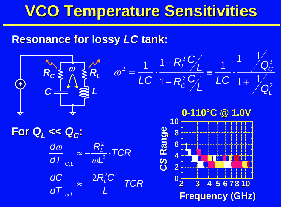
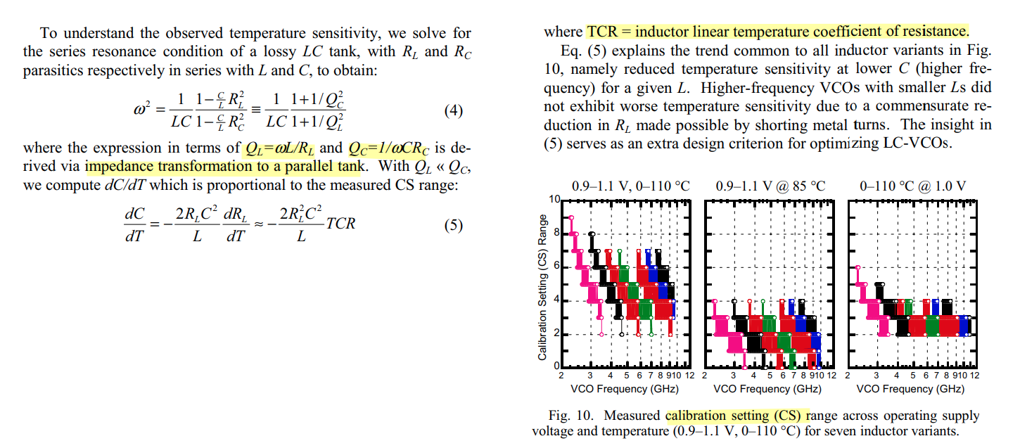
\[ \omega=\frac{1}{\sqrt{L_p C_p}} = \frac{1}{\sqrt{L_s\frac{Q_L^2+1}{Q_L^2} C_s\frac{Q_C^2}{Q_C^2+1}}} = \frac{1}{\sqrt{L_sC_s}}\cdot \sqrt{\frac{1+1/Q_c^2}{1+1/Q_L^2}} \] Assuming the tank's Q is limited by the inductor's quality factor \(Q_L\), i.e. \(Q_L\ll Q_c\) \[ \omega\approx \frac{1}{\sqrt{L_sC_s}}\cdot \sqrt{1-\frac{1}{Q_L^2}} =\omega_0\cdot\sqrt{1-\frac{1}{Q_L^2}} = \omega_0\cdot\sqrt{1-\frac{C R_L^2}{L}} \] where \(\omega_0=\frac{1}{\sqrt{L_sC_s}}\) is the first order approximation of the resonant frequency
Expand:
\[ \boxed{ \omega^2 \approx \frac{1}{LC} - \frac{R_L^2}{L^2} } \]
This form makes the derivation especially simple.
How much must \(C\) change with temperature to keep the VCO resonance frequency \(\omega\) constant as \(R_L\) changes with temperature?
The calibration capacitor compensates temperature drift, so during compensation \(\color{red}\frac{d\omega}{dT}=0.\)
Assume also that \(L\)'s temperature variation is much smaller than the effect of \(R_L\), so \(L\) is treated as constant.
Differentiate \(\omega^2\) with respect to \(T\):
\[ 0 = \frac{d}{dT} \left[ \frac{1}{LC} - \frac{R_L^2}{L^2} \right]. \]
Hence
\[ \color{red}\boxed{ \frac{dC}{dT} = -\frac{2R_LC^2}{L} \frac{dR_L}{dT} } \tag{5a} \]
which is the first part of Eq. (5).
The inductor's temperature coefficient of resistance is
\[ \boxed{ TCR = \frac{1}{R_L}\frac{dR_L}{dT} } \]
so
\[ \frac{dR_L}{dT} = R_L\,TCR. \]
Substitute this into (5a):
\[ \frac{dC}{dT} = -\frac{2R_LC^2}{L} (R_L TCR), \]
giving
\[ \boxed{ \frac{dC}{dT} \approx -\frac{2R_L^2C^2}{L}\,TCR } \tag{5} \]
which is exactly the paper's equation.
Also, the negative sign has a physical meaning: for a metal inductor,
\[ T\uparrow \Rightarrow R_L\uparrow, \]
and from
\[ \omega^2 \approx \frac{1}{LC}-\frac{R_L^2}{L^2}, \]
increased \(R_L\) tends to reduce \(\omega\). To maintain the same \(\omega\), you need
\[ \boxed{C\downarrow} \]
hence \(dC/dT<0\).
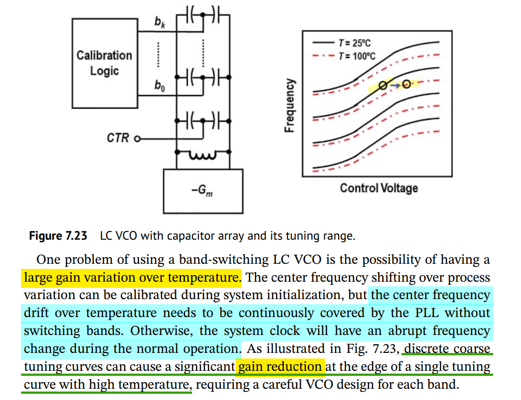
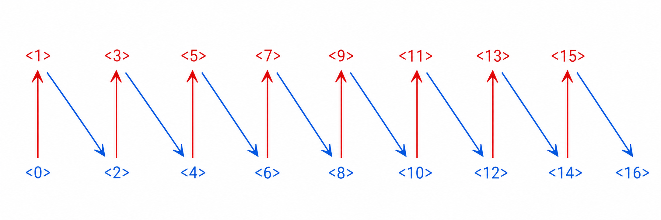
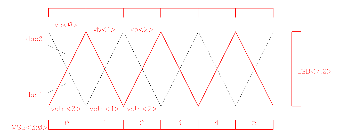
continuous coding to eliminate glitch during code changing
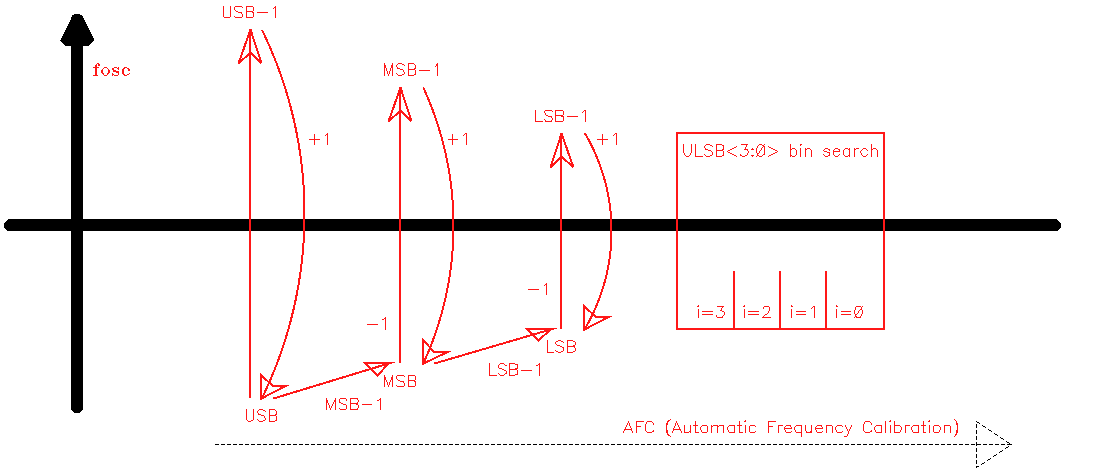
Automatic Frequency Control
Inverter-19 - Ring Oscillators and Process Variations [https://youtu.be/b1xZU0aD4hA]
IC_designer, VCO cali [link]

Asynchronous clock alignment results in a maximum skew of \(\pm 1\) cycle (\(\Delta \in [-1, 1]\))
\[ (N+\Delta) T_o = MT_r\quad \Delta\in [-1,1] \]
then,
\[ f_o = \frac{N}{M}f_r\color{red}\left(1+\frac{\Delta}{N}\right) \]
\(\frac{\Delta}{N}\) determine measurement accuracy, \(\frac{\Delta}{N} \lt 0.01\) if 1% accuracy is needed
Automatic Amplitude Control (AAC)
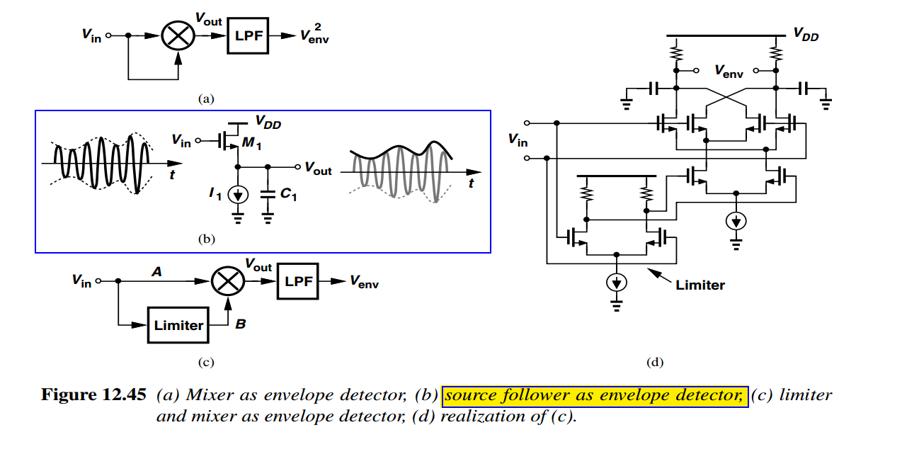
peak detector, envelope detector
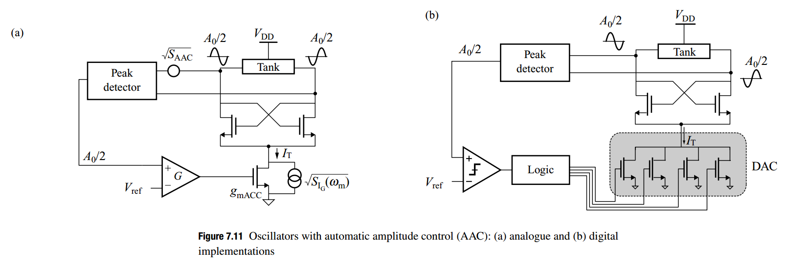
The digital AAC regulates the amplitude without increasing the amplitude modulation noise

PN Reduction Techniques
Y. Hu, T. Siriburanon and R. B. Staszewski, "Oscillator Flicker Phase Noise: A Tutorial," in IEEE Transactions on Circuits and Systems II: Express Briefs, vol. 68, no. 2, pp. 538-544, Feb. 2021 [paper] [slides]
Tank current Harmonics
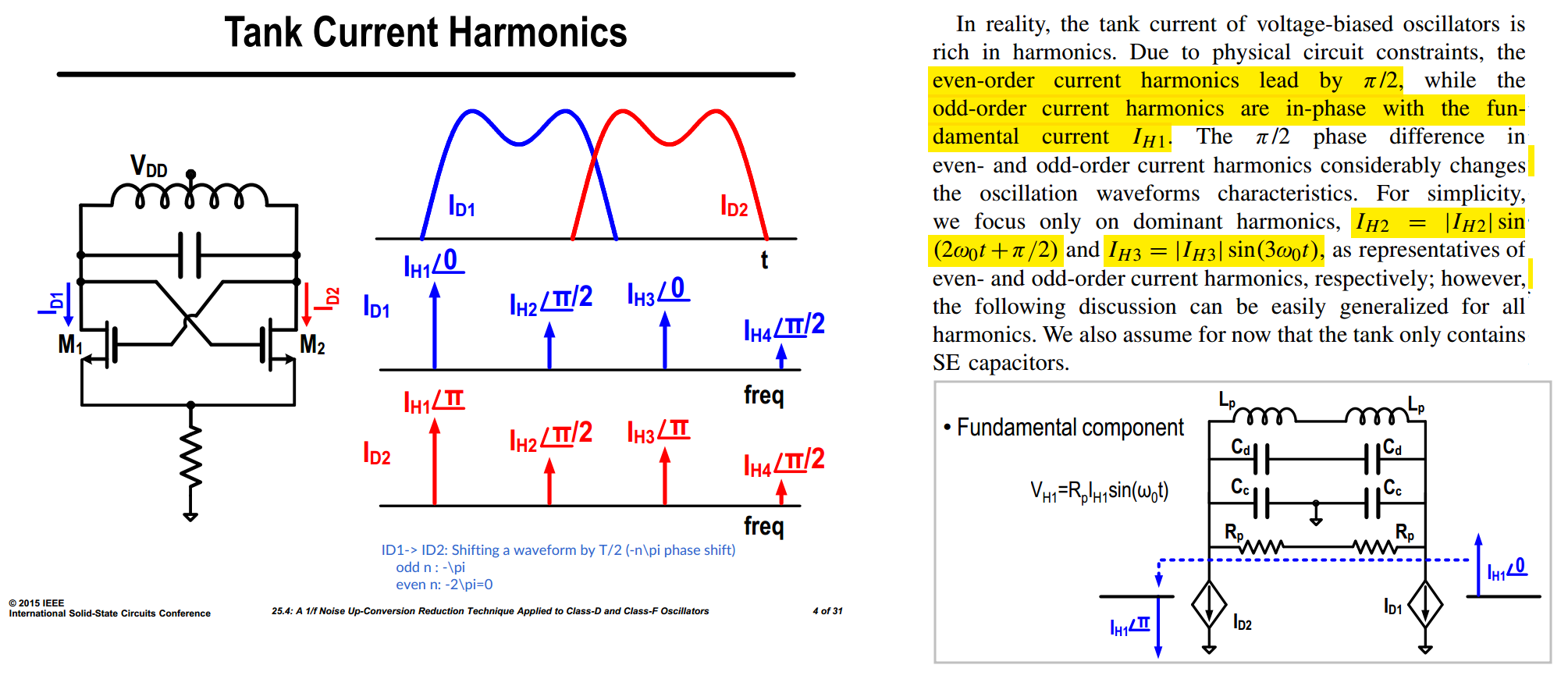
Due to MOS nonlinearity

with \(\boxed{x(t) = \sin(\omega_0 t)}\) \[ y_{\sin}(t) = \alpha_1 \sin(\omega_0 t)+ \alpha_2\frac{1-\cos(2\omega_0t)}{2} + \alpha_3 \frac{3\sin(\omega_0 t) -\sin(3\omega_0 t)}{4} +\alpha_4\frac{3-4\cos(2\omega_0 t)+\cos(4\omega_0 t)}{8} \]
and using \(\cos \theta = \sin(\theta + \pi/2)\)
\[ y_{\sin}(t) = \underbrace{\frac{\alpha_2}{2} + \frac{3\alpha_4}{8}}_{\text{DC}} + \underbrace{\left(\alpha_1 + \frac{3\alpha_3}{4}\right)\sin(\omega_0 t)}_{\omega_0} - \underbrace{\frac{\alpha_2 + \alpha_4}{2}\,\sin\!\left(2\omega_0 t + \textcolor{blue}{\frac{\pi}{2}}\right)}_{2\omega_0} - \underbrace{\frac{\alpha_3}{4}\,\sin(3\omega_0 t)}_{3\omega_0} + \underbrace{\frac{\alpha_4}{8}\,\sin\!\left(4\omega_0 t + \textcolor{blue}{\frac{\pi}{2}}\right)}_{4\omega_0} \]
with \(\boxed{x(t) = \sin(-\omega_0 t)}\) and we have \(\sin\left(-\alpha+\frac{\pi}{2}\right) = \sin\left(\alpha+\frac{\pi}{2}\right)\), \(\sin(-\alpha) = \sin(\alpha +\pi)\) \[ y_{-\sin}(t) = \underbrace{\frac{\alpha_2}{2} + \frac{3\alpha_4}{8}}_{\text{DC}} + \underbrace{\left(\alpha_1 + \frac{3\alpha_3}{4}\right)\sin(\omega_0 t+\textcolor{red}{\pi})}_{\omega_0} - \underbrace{\frac{\alpha_2 + \alpha_4}{2}\,\sin\!\left(2\omega_0 t + \textcolor{blue}{\frac{\pi}{2}}\right)}_{2\omega_0} - \underbrace{\frac{\alpha_3}{4}\,\sin(3\omega_0 t+\textcolor{red}{\pi})}_{3\omega_0} + \underbrace{\frac{\alpha_4}{8}\,\sin\!\left(4\omega_0 t + \textcolor{blue}{\frac{\pi}{2}}\right)}_{4\omega_0} \]
with \(\boxed{x(t) = \cos(\omega_0 t)}\) \[ y_{\cos}(t) = \underbrace{\frac{\alpha_2}{2}+\frac{3\alpha_4}{8}}_{\text{DC}} + \underbrace{\left(\alpha_1+\frac{3\alpha_3}{4}\right)\cos(\omega_0 t)}_{\omega_0} + \underbrace{\frac{\alpha_2+\alpha_4}{2}\cos(2\omega_0 t)}_{2\omega_0} + \underbrace{\frac{\alpha_3}{4}\cos(3\omega_0 t)}_{3\omega_0} + \underbrace{\frac{\alpha_4}{8}\cos(4\omega_0 t)}_{4\omega_0} \] They're the same waveform; one is the other shifted in time by a quarter of the fundamental period: \[ y_{\cos}(t) = y_{\sin}\!\left(t + \frac{T}{4}\right), \qquad T = \frac{2\pi}{\omega_0} \]
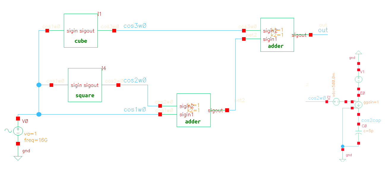
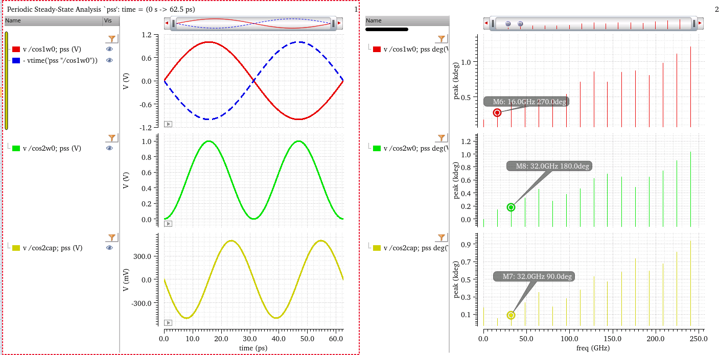
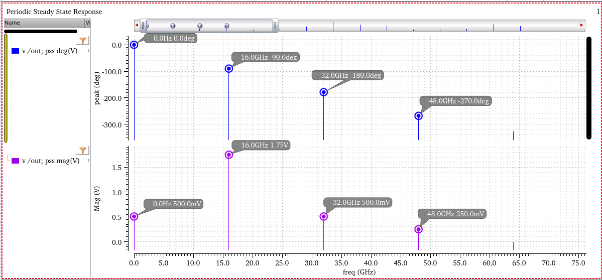
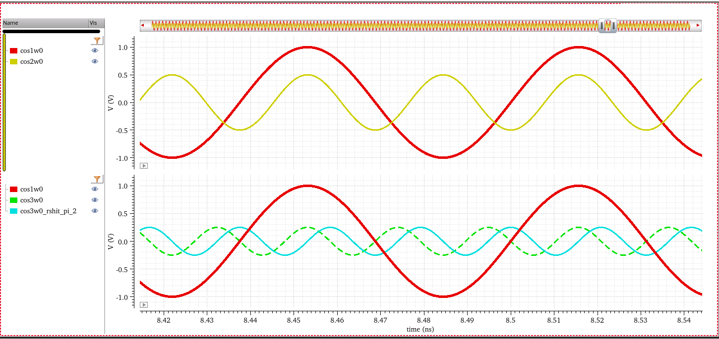
Given \(\Delta t\) is constant \[
\boxed{\Delta t = \frac{\Delta\Phi_N}{N\omega_0} \implies \Delta\Phi_N =
N\Delta\Phi_0 \quad (\Delta t = \text{constant})}
\] 
Harmonic Shaping (Common-Mode Resonance)
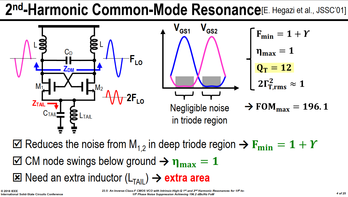
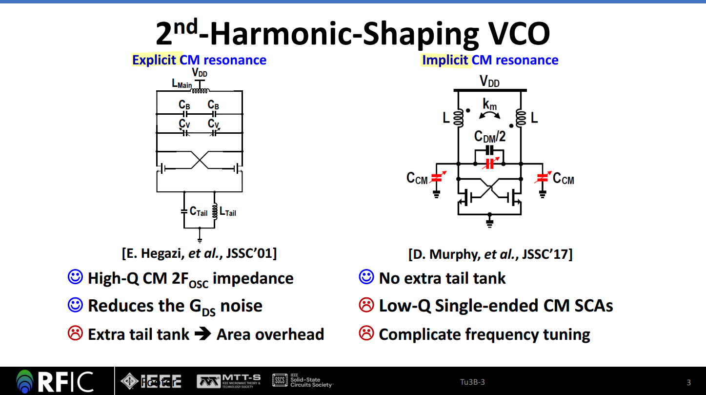
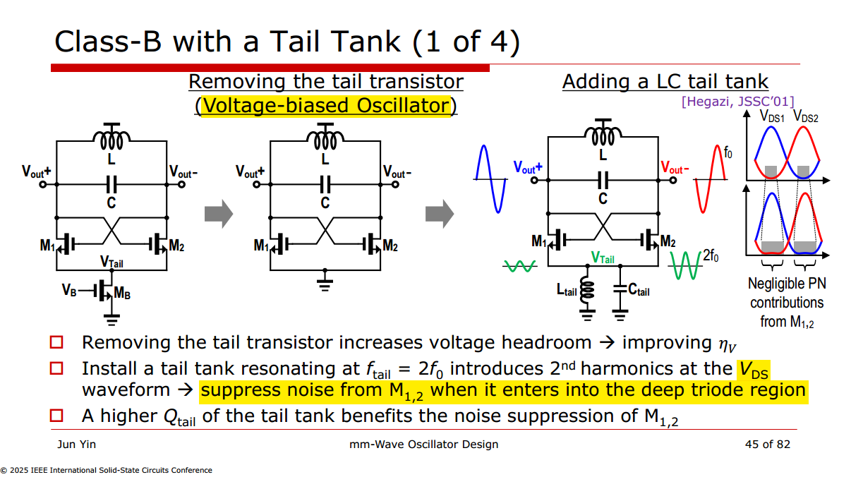
E. Hegazi, H. Sjoland and A. Abidi, "A filtering technique to lower oscillator phase noise," 2001 IEEE International Solid-State Circuits Conference. Digest of Technical Papers. ISSCC (Cat. No.01CH37177), San Francisco, CA, USA, 2001 [paper, slides]
—, "A filtering technique to lower LC oscillator phase noise," in IEEE Journal of Solid-State Circuits, vol. 36, no. 12, pp. 1921-1930, Dec. 2001 [https://people.engr.tamu.edu/spalermo/ecen620/filtering_tech_lc_osc_hegazi_jssc_2001.pdf]
A. Bevilacqua and P. Andreani, "An Analysis of 1/f Noise to Phase Noise Conversion in CMOS Harmonic Oscillators," in IEEE Transactions on Circuits and Systems I: Regular Papers, vol. 59, no. 5, pp. 938-945, May 2012
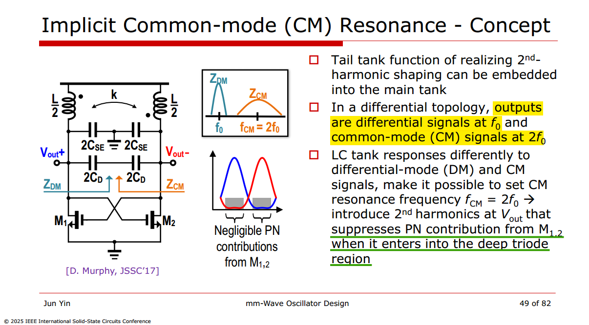
D. Murphy, H. Darabi and H. Wu, "Implicit Common-Mode Resonance in LC Oscillators," in IEEE Journal of Solid-State Circuits, vol. 52, no. 3, pp. 812-821, March 2017, [https://sci-hub.st/10.1109/JSSC.2016.2642207]
—, "25.3 A VCO with implicit common-mode resonance," 2015 IEEE International Solid-State Circuits Conference - (ISSCC) Digest of Technical Papers, San Francisco, CA, USA, 2015 [https://sci-hub.st/10.1109/ISSCC.2015.7063116]
M. Shahmohammadi, M. Babaie and R. B. Staszewski, "25.4 A 1/f noise upconversion reduction technique applied to Class-D and Class-F oscillators," 2015 IEEE International Solid-State Circuits Conference - (ISSCC) Digest of Technical Papers, San Francisco, CA, USA, 2015 [https://sci-hub.ru/10.1109/ISSCC.2015.7063117]
—, "A 1/f Noise Upconversion Reduction Technique for Voltage-Biased RF CMOS Oscillators," in IEEE Journal of Solid-State Circuits, vol. 51, no. 11, pp. 2610-2624, Nov. 2016 [https://pure.tudelft.nl/ws/portalfiles/portal/30880387/07571191.pdf]
Michael Perrott August 12, 2008, Short Course On Phase-Locked Loops and Their Applications Day 2, AM Lecture Basic Building Blocks Voltage-Controlled Oscillators [https://www.cppsim.com/PLL_Lectures/day2_am.pdf]
Yunbo Huang, Zunsong Yang, et al., "A 7.0-to-8.6GHz Balanced Class-F-1 VCO with a Trifilar Transformer-Based Tank Achieving 194.5dBc/Hz FoM," IEEE MTT-S Radio Frequency Integrated Circuits (RFIC), June 2026
credits to Claude Opus 5.5
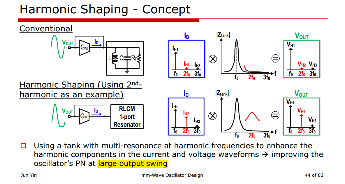
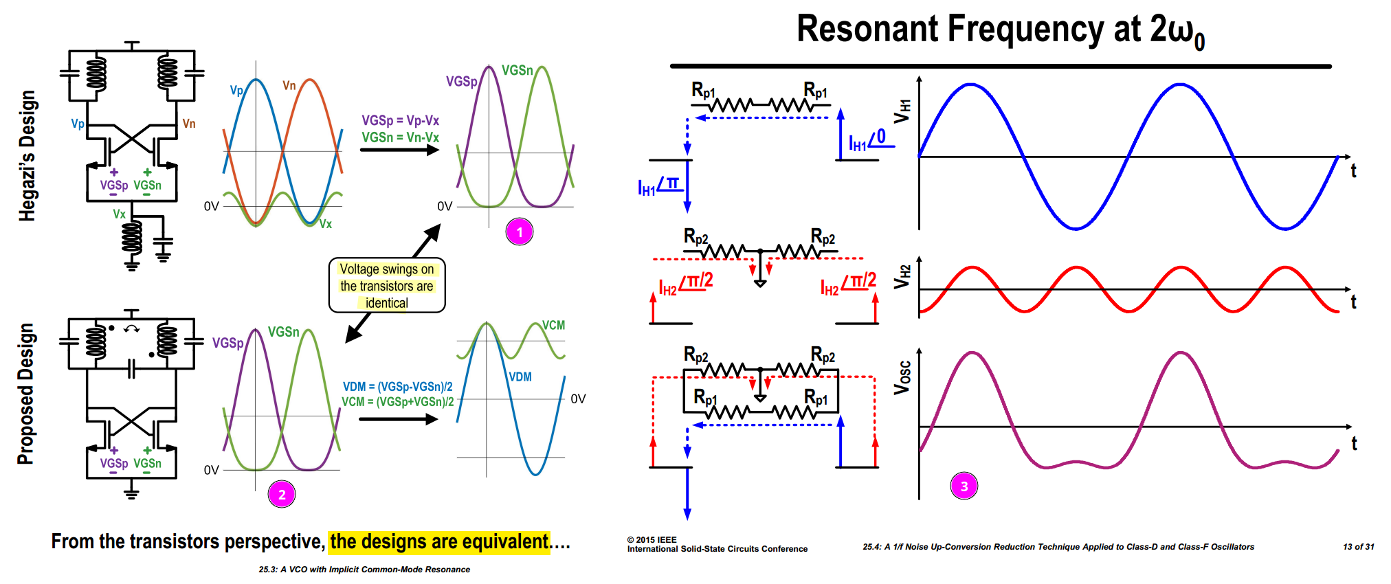
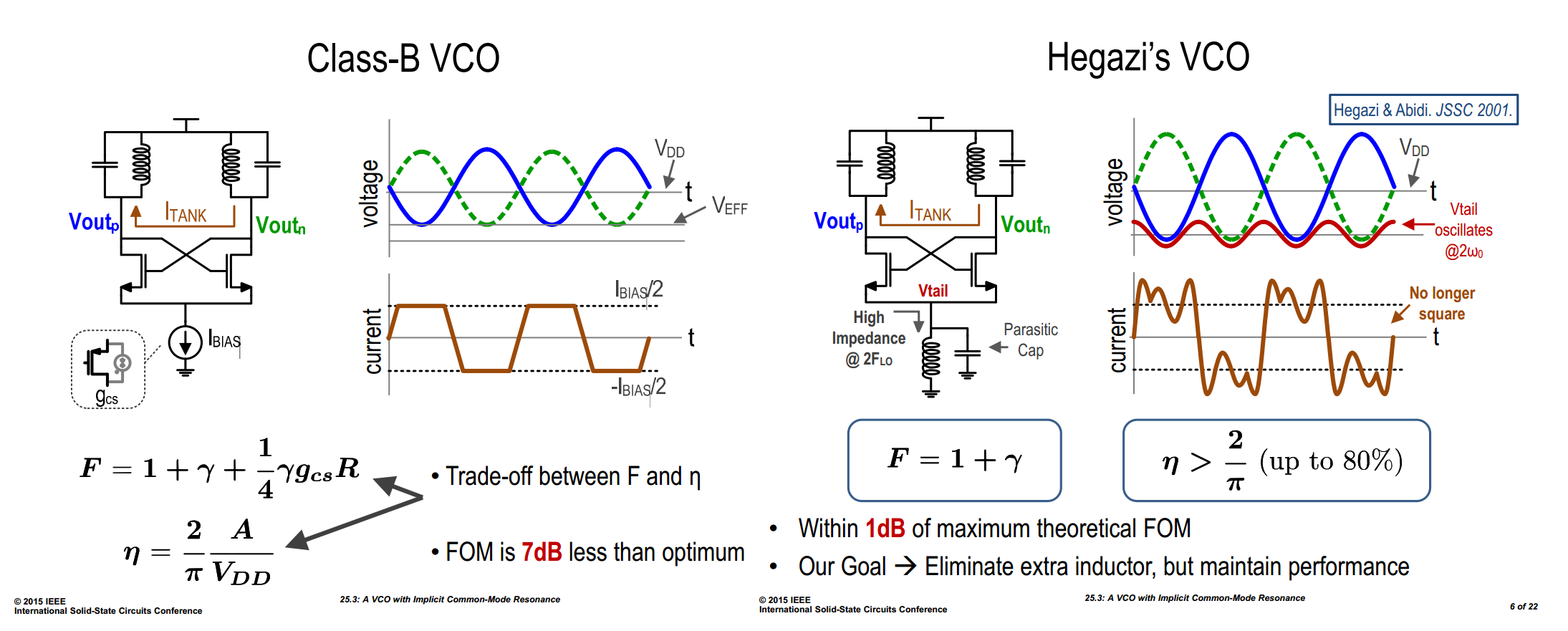
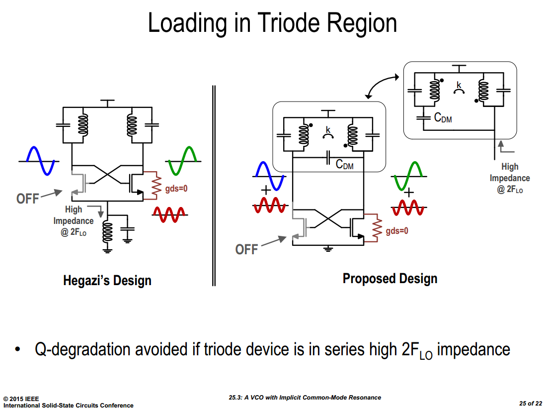
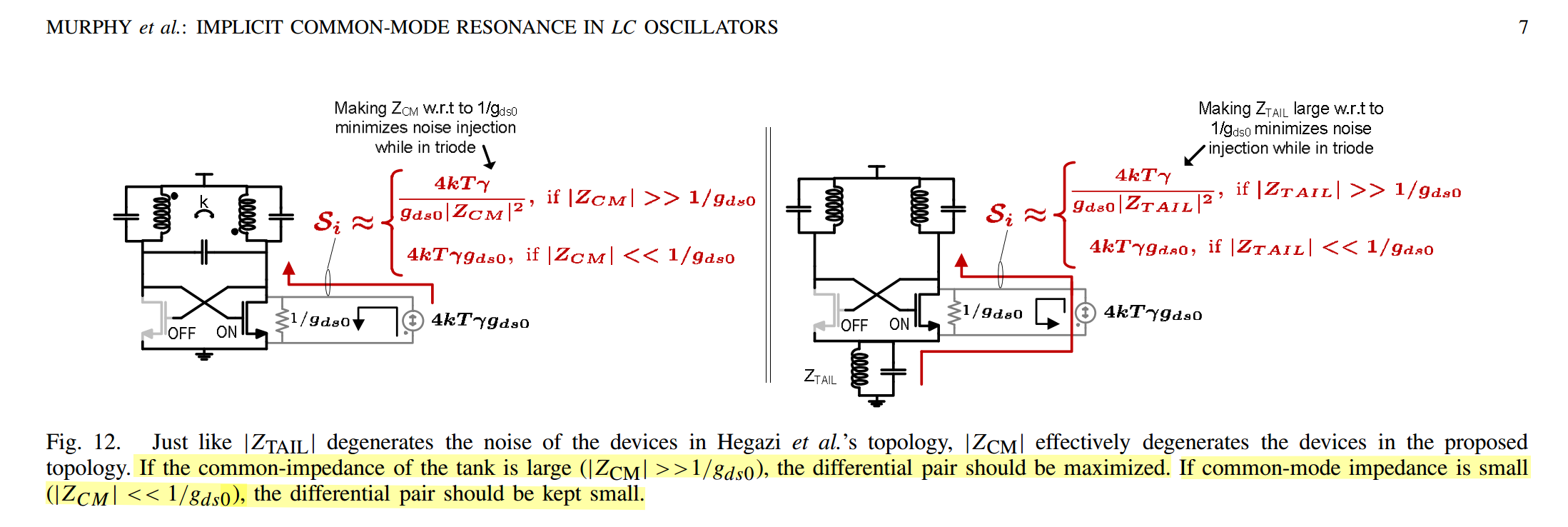
Give the common-mode (CM) loop a high, resistive impedance at \(2f_0\), \(Z_{2f_0}\): either \(Z_S\) in the tail (explicit, Hegazi: \(L_\text{tail}\) resonates the common-source capacitance at \(2f_0\)) or \(Z_{CM}\) in the tank's CM path (implicit, Murphy, Shahmohammadi: CM resonance of the main tank). Either way the transistors see the same \(V_{GS}\) and \(V_{DS}\)

- Triode loading and thermal noise (\(1/f^2\) region): when the ON device enters deep triode, its \(1/g_{ds0}\), a noisy resistor (\(\gamma \to 1\)), sits in series with \(Z_{2f_0}\), which suppresses its loss and its noise together: it no longer de-Qs the tank, and the noise reaching the tank drops to \(S_i \approx 4kT\gamma/(g_{ds0}\lvert Z_{2f_0}\rvert^2)\). The impedance matters at \(2f_0\) because the two FETs take turns in triode: two events per period on a CM node. Loss matters more than noise here: triode sits at the waveform extremes, where the ISF \(\approx 0\). With \(V \propto \cos\omega_0 t\) and triode conductance \(g(t)\), the loss scales as \(\langle g\cos^2\omega_0 t\rangle\) but the PM noise as \(\langle g\sin^2\omega_0 t\rangle\); a uniform \(\pm 60^\circ\) triode window gives about \(0.4\times\) the PM noise of a fixed resistor with the same loss
- Flicker upconversion (\(1/f^3\) region): \(I_{H2}\) is \(\pi/2\) away from \(I_{H1}\). A resistive \(2f_0\) impedance keeps \(V_{H2}\) at that phase, so the single-ended \(V_{GS}\) and \(V_{DS}\) rise and fall symmetrically and \(\Gamma_\text{eff,dc} = 0\). The capacitive path of a plain tank adds another \(-\pi/2\), the waveform turns asymmetric and \(\Gamma_\text{eff,dc} \neq 0\). Energy view: \(H_2\) no longer flows through a capacitor (the tail filter blocks it, or \(R_{p2}\) absorbs it), so it adds no Groszkowski shift for \(1/f\) noise to modulate
The two benefits pull the \(Q\) of the \(2f_0\) resonance in opposite directions
| triode / thermal | flicker | |
|---|---|---|
| needs | \(\lvert Z_{2f_0}\rvert \gg 1/g_{ds0}\) | \(\angle Z_{2f_0} \approx 0\) |
| detuning | tolerant | must be tuned closely |
| \(Q\) at \(2f_0\) | high helps | low is more robust |
A mistuned high-Q CM tank can be worse than none: Shahmohammadi's 5 GHz voltage-biased class-B (\(Q_{DM}=10\), \(Q_{CM}=20\)) has a \(1/f^3\) corner of ~10 kHz when tuned, 1.1 MHz at \(\omega_{CM}=1.7\,\omega_{DM}\), and 400 kHz without the technique. Hence the adaptive CM-resonance tuning in Gallucci (JSSC'25)
S. Gallucci et al., "A Low-Noise Digital PLL With an Adaptive Common-Mode Resonance Tuning Technique for Voltage-Biased Oscillators," in IEEE Journal of Solid-State Circuits, vol. 60, no. 12, pp. 4572-4586, Dec. 2025 P. Liu et al., "A 128Gb/s ADC/DAC Based PAM-4 Transceiver with >45dB Reach in 3nm FinFET," 2025 Symposium on VLSI Technology and Circuits (VLSI Technology and Circuits), Kyoto, Japan, 2025
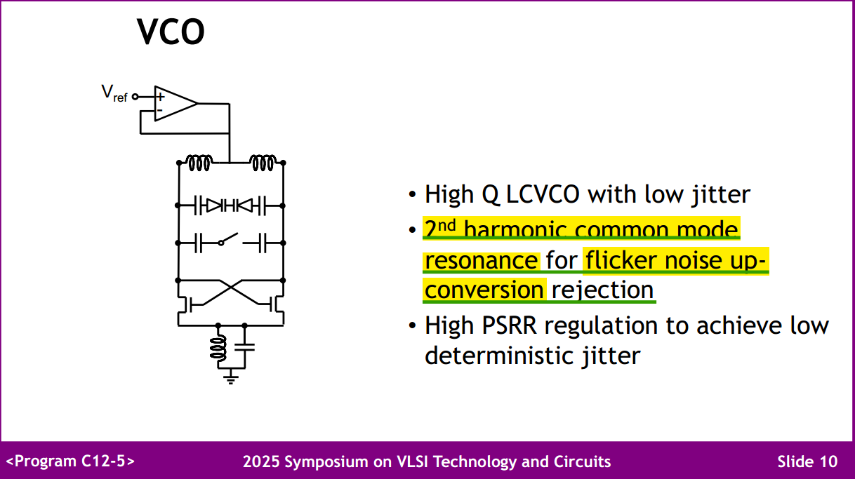
Narrowing of conduction angle
Y. Hu, T. Siriburanon and R. B. Staszewski, "Intuitive Understanding of Flicker Noise Reduction via Narrowing of Conduction Angle in Voltage-Biased Oscillators," in IEEE Transactions on Circuits and Systems II: Express Briefs, vol. 66, no. 12, pp. 1962-1966, Dec. 2019 [https://sci-hub.se/10.1109/TCSII.2019.2896483]
TODO 📅
Gate-drain phase shift
TODO 📅
Supply Sensitivity in LC Oscillators
Y. Chen et al., "A Supply Pushing Reduction Technique for LC Oscillators Based on Ripple Replication and Cancellation," in IEEE Journal of Solid-State Circuits, vol. 54, no. 1, pp. 240-252, Jan. 2019 [https://sci-hub.ru/10.1109/JSSC.2018.2871195]
R. Yang, R. B. Staszewski, M. Babaie and Z. Zong, "Passive Techniques to Reduce Supply Sensitivity in an LC Oscillator Achieving 46-dB Suppression," 2025 IEEE European Solid-State Electronics Research Conference (ESSERC), Munich, Germany, 2025, pp. 509-512, doi: 10.1109/ESSERC66193.2025.11214006
—, "Fully Passive Techniques for Reducing Supply Sensitivity in LC Oscillators," in IEEE Open Journal of the Solid-State Circuits Society, doi: 10.1109/OJSSCS.2026.3723352 [https://ieeexplore.ieee.org/stamp/stamp.jsp?tp=&arnumber=11653291]
TODO 📅
simulation in oscillator
varactor simulation
Three methods:
- PSS +PSP (pay attention to port termination and voltage amplitude)
- PSS +PAC
- PSS Only
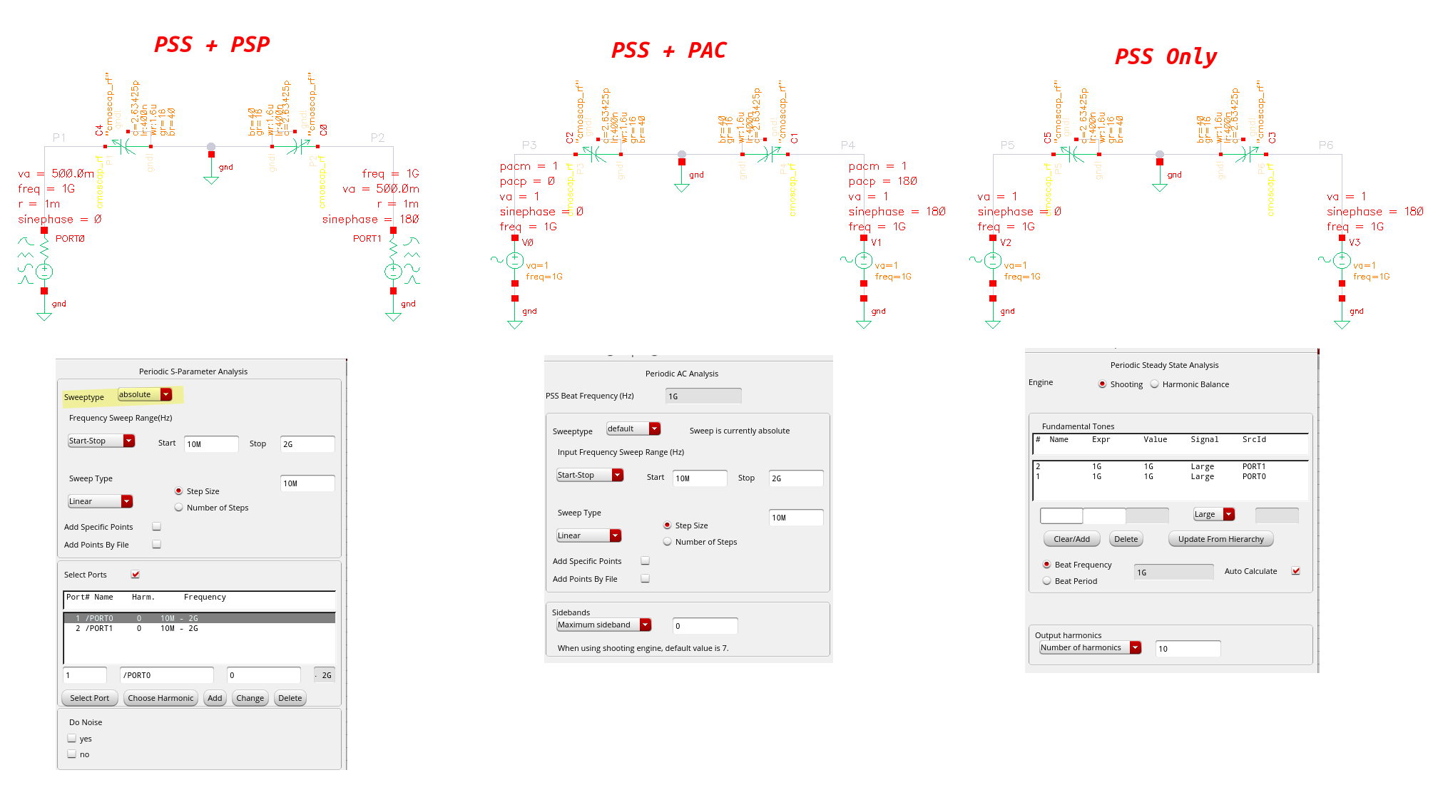
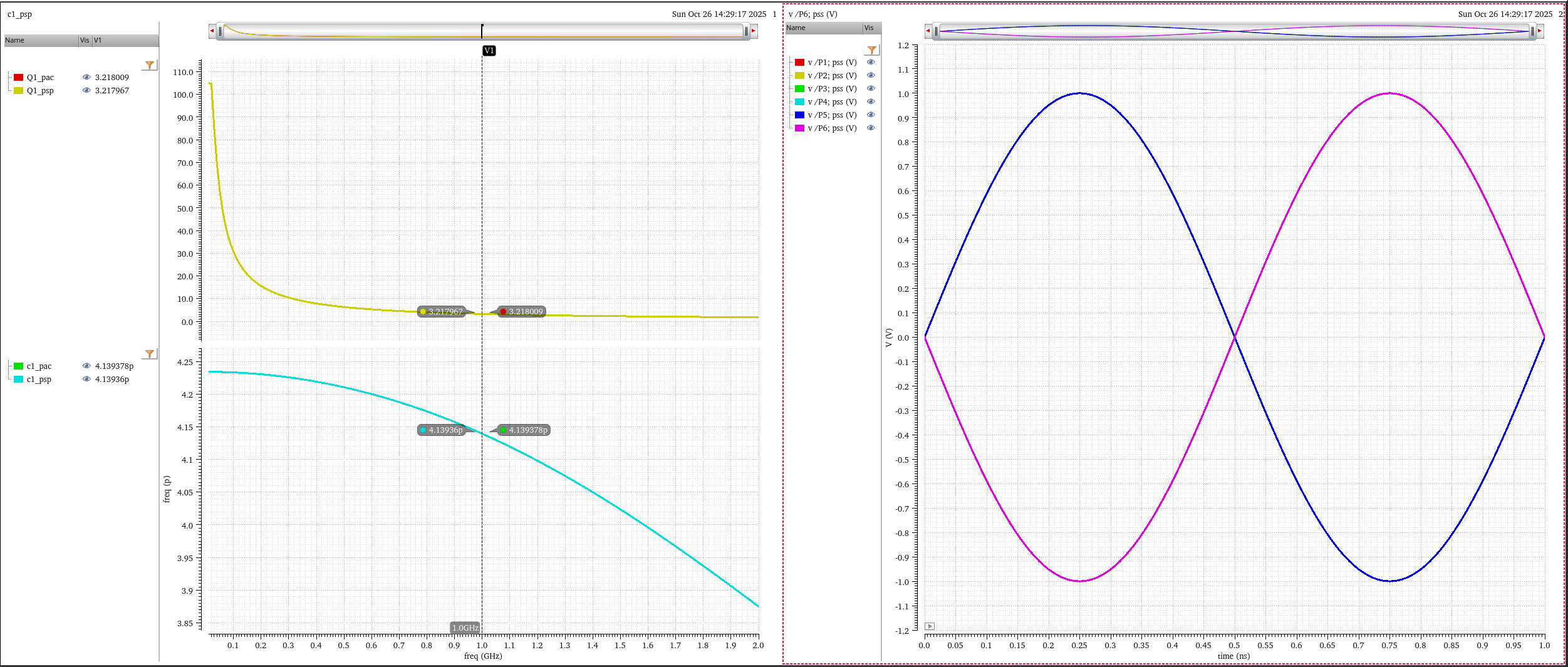
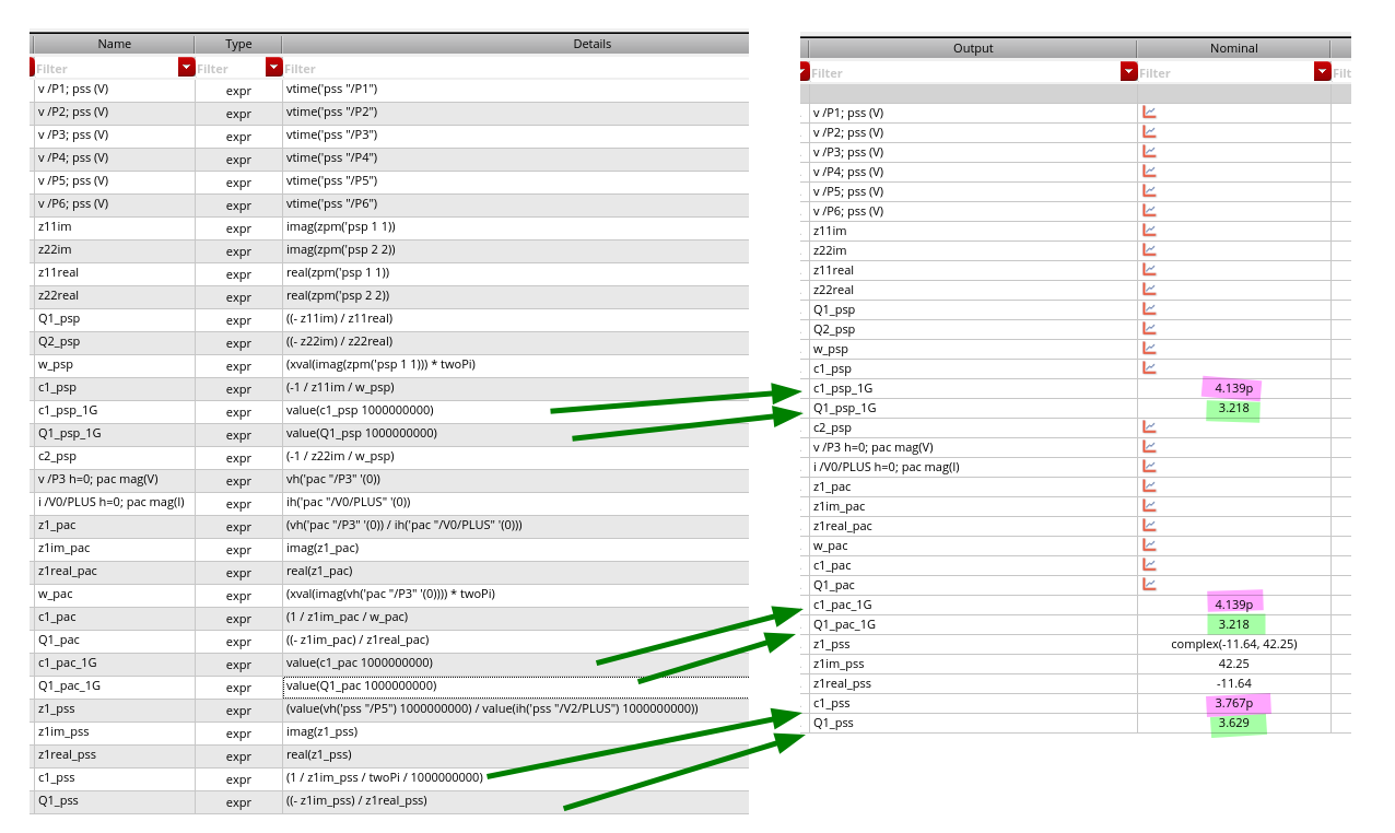
rms only scale magnitude \(1/\sqrt{2}\) but retain phase for complex
number, like harmonic
mag(vh('pss "/P5"))=mag(rms(vh('pss "/P5"))) * (2**0.5)phaseDegUnwrapped(vh('pss "/P5"))=phaseDegUnwrapped(rms(vh('pss "/P5")))

reference
Pietro Andreani. ISSCC 2011 T1: Integrated LC oscillators
—. ISSCC 2017 F2: Integrated Harmonic Oscillators
—. SSCS Distinguished Lecture: RF Harmonic Oscillators Integrated in Silicon Technologies [https://www.ieeetoronto.ca/wp-content/uploads/2020/06/DL-Toronto.pdf]
—. ESSCIRC 2019 Tutorials: RF Harmonic Oscillators Integrated in Silicon Technologies [https://youtu.be/k1I9nP9eEHE]
—. "Harmonic Oscillators in CMOS—A Tutorial Overview," in IEEE Open Journal of the Solid-State Circuits Society, vol. 1, pp. 2-17, 2021 [https://ieeexplore.ieee.org/stamp/stamp.jsp?tp=&arnumber=9530265]
A. A. Abidi and D. Murphy, "How to Design a Differential CMOS LC Oscillator," in IEEE Open Journal of the Solid-State Circuits Society, vol. 5, pp. 45-59, 2025 [https://ieeexplore.ieee.org/stamp/stamp.jsp?arnumber=10818782]
C. Samori, "Tutorial: Understanding Phase Noise in LC VCOs," 2016 IEEE International Solid-State Circuits Conference (ISSCC), San Francisco, CA, USA, 2016
—, "Understanding Phase Noise in LC VCOs: A Key Problem in RF Integrated Circuits," in IEEE Solid-State Circuits Magazine, vol. 8, no. 4, pp. 81-91, Fall 2016 [https://sci-hub.se/10.1109/MSSC.2016.2573979]
—, Phase Noise in LC Oscillators: From Basic Concepts to Advanced Topologies [https://www.ieeetoronto.ca/wp-content/uploads/2020/06/DL-VCO-short.pdf]
Jun Yin. ISSCC 2025 T10: mm-Wave Oscillator Design
Peter Kinget, ISSCC 2010 short course, Transistor-Level Design of Critical PLL Circuits
J. Bank, "A harmonic-oscillator design methodology based on describing functions," Ph.D. dissertation, Dept. Signals Syst., Sch. Elect. Eng., Chalmers Univ. Techn., Chalmers, Sweden, 2006. [https://publications.lib.chalmers.se/records/fulltext/17376.pdf]
Waleed Khalil, CICC2021 ES2-3: VCO Design Challenges and Solutions for mm-wave Applications
Razavi, Behzad. RF Microelectronics. 2nd ed. Prentice Hall, 2012.
—. Design of CMOS Phase-Locked Loops: From Circuit Level to Architecture Level. Cambridge University Press; 2020.
Lacaita, Andrea Leonardo, Salvatore Levantino, and Carlo Samori. Integrated frequency synthesizers for wireless systems. Cambridge University Press, 2007
M. Babaie, M. Shahmohammadi, R. B. Staszewski, (2019) "RF CMOS Oscillators for Modern Wireless Applications" River Publishers [https://www.riverpublishers.com/pdf/ebook/RP_E9788793609488.pdf]
Luong, H. C., & Yin, J. (2016). Transformer-based design techniques for oscillators and frequency dividers. Springer International Publishing
Darabi H. Radio Frequency Integrated Circuits and Systems. 2nd ed. Cambridge University Press; 2020.
Manetakis, K. (2023). Topics in LC Oscillators: Principles, phase noise, pulling, inductor design. Springer Nature Switzerland Springer. [eetop link]
Hajimiri, A., & Lee, T. H. (1999). The design of low noise oscillators. Norwell, MA: Kluwer
Hegazi, Emad, Asad Abidi, and Jacob Rael. The Designer's Guide to High-purity Oscillators. [New York]: Kluwer Academic Publishers, 2005.
Rhee, Woogeun, and Zhiping Yu. Phase-Locked Loops: System Perspectives and Circuit Design Aspects. John Wiley & Sons, 2024.