Link Models

Posted on 2025-11-29 Edited on 2026-04-11 In link

Time domain modeling

While many different analysis methods exist, including frequency and statistical analysis, time domain results remain the final sign-off

serdespy

Richard Barrie. serdespy — A python library for system-level SerDes modelling and simulation [https://github.com/richard259/serdespy]

—, Microelectronics [Introduction to SerDesPy], [Simple Channel Modeling Example with SerDesPy], [Modelling Equalization with SerDesPy]
1
2
3
# Python 3.10
pip install samplerate
pip install 'numpy<2.0.0'

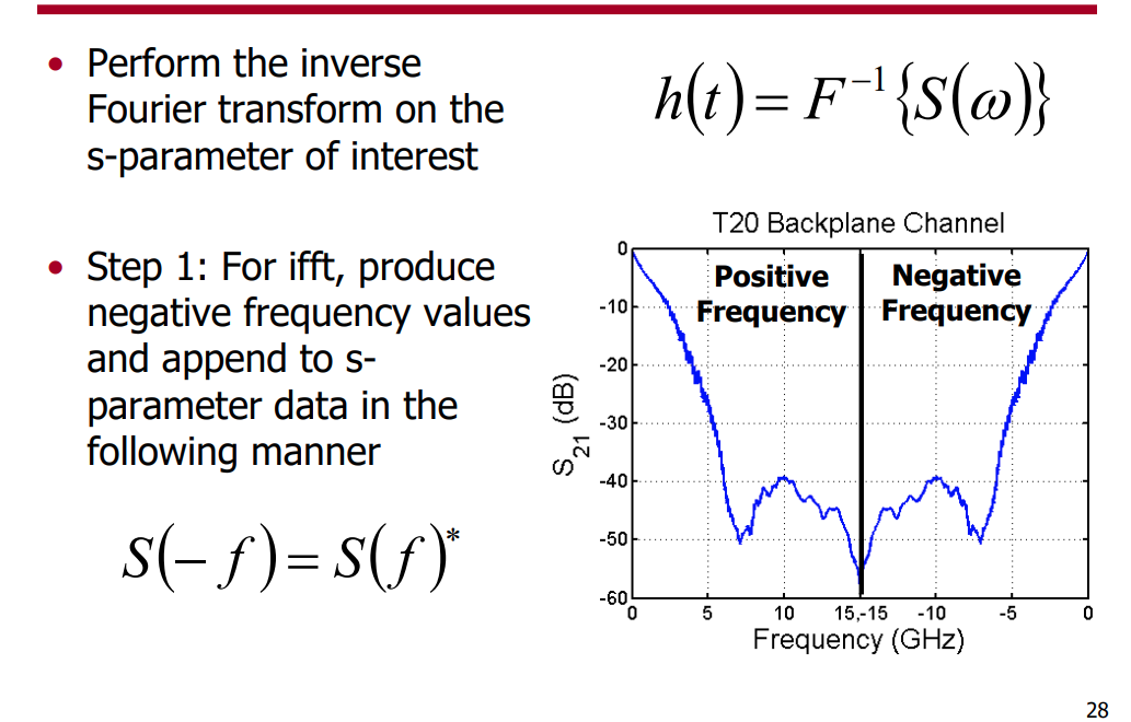
ifft of sampling continuous-time transfer function

freq2impulse.drawio

def freq2impulse(H, f):
    #Returns the impulse response, h, and (optionally) the step response,
    #hstep, for a system with complex frequency response stored in the array H
    #and corresponding frequency vector f.  The time array is
    #returned in t.  The frequency array must be linearly spaced.

    Hd = np.concatenate((H,np.conj(np.flip(H[1:H.size-1]))))
    h = np.real(np.fft.ifft(Hd))
    #hstep = sp.convolve(h,np.ones(h.size))
    #hstep = hstep[0:h.size]
    t= np.linspace(0,1/f[1],h.size+1)
    t = t[0:-1]

    return h,t

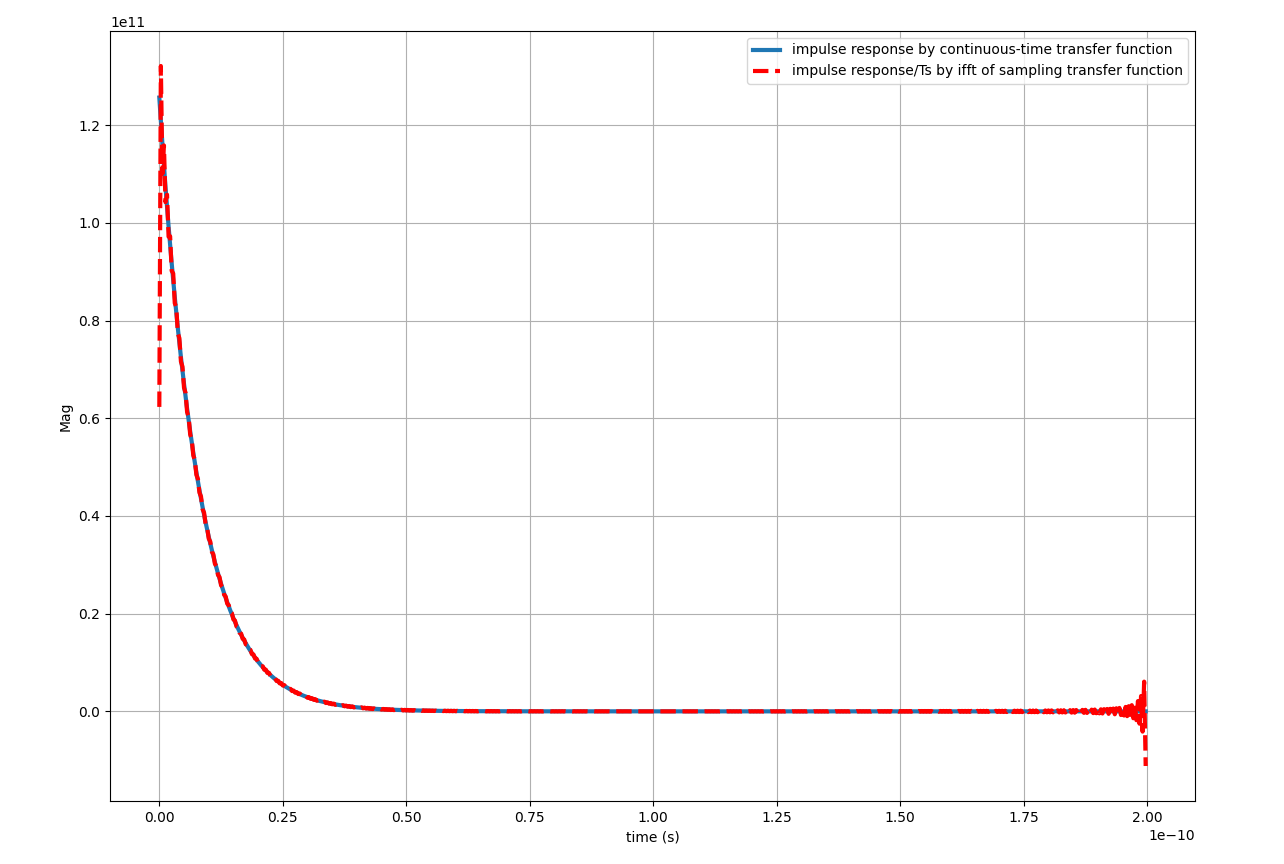
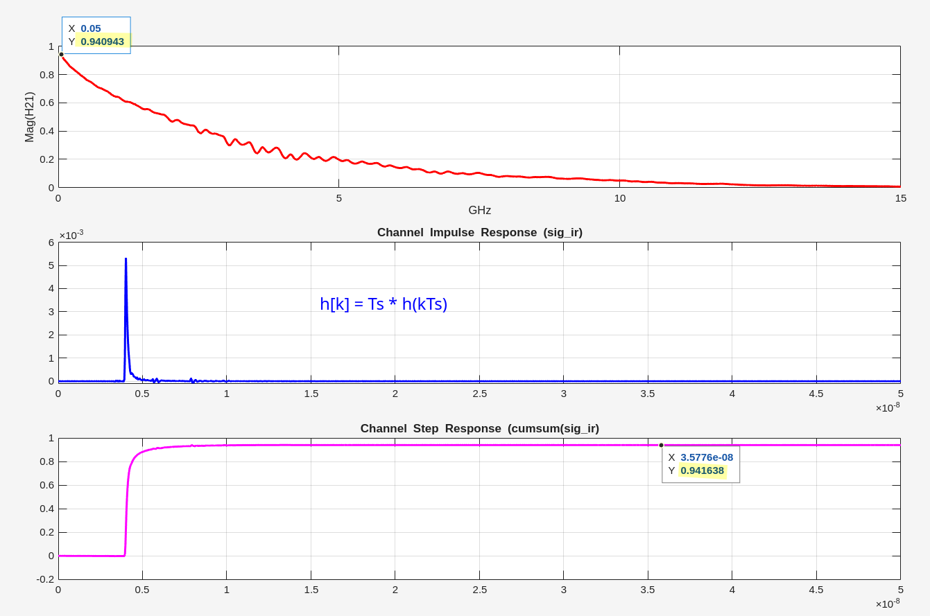
Maybe, the more straightforward method is sampling impulse response of continuous-time transfer function directly

import numpy as np
from scipy import signal
import matplotlib.pyplot as plt

fbw = 20e9
wbw = fbw * 2 * np.pi
samples_per_symbol = 64
UI = 1/50e9
Ts = UI/samples_per_symbol
fs = 1/Ts
ws = fs * 2 * np.pi
ttot = 4/fbw # heuristic
N = int(0.5 * fs * ttot)+1
w, H = signal.freqs([1], [1/wbw, 1], np.linspace(0, 0.5*ws, N))

## freq2impulse(H, f), ifft - using sample of continuous-time tranfer function
f = w/(2*np.pi)
Hd = np.concatenate((H,np.conj(np.flip(H[1:H.size-1]))))
hd = np.real(np.fft.ifft(Hd))
t= np.linspace(0,1/f[1],hd.size+1)
t = t[0:-1]

## continuous-time transfer function - impulse
t, hc = signal.impulse(([1], [1/wbw, 1]), T = t)

## hd(kTs) = Ts*hc(kTs)
plt.figure(figsize = (14,10))
plt.plot(t, hc, t, hd/Ts, '--r', linewidth=3)
plt.grid(); plt.legend(['impulse response by continuous-time transfer function','impulse response/Ts by ifft of sampling transfer function'])
plt.ylabel('Mag'); plt.xlabel('time (s)'); plt.show()

import scipy as sp


#time per bit
UI = 1/data_rate

#define oversample ratio
samples_per_symbol = 64

#timestep
dt = UI/samples_per_symbol

#oversampled signal
signal_ideal = np.repeat(signal_BR, samples_per_symbol)

#eye diagram of ideal signal
sdp.simple_eye(signal_ideal, samples_per_symbol*3, 100, dt, "{}Gbps 2-PAM Signal".format(data_rate/1e9),linewidth=1.5, res=200)

#max frequency for constructing discrete transfer function
max_f = 1/dt

#max_f in rad/s
max_w = max_f*2*np.pi

#heuristic to get a reasonable impulse response length
ir_length = int(4/(freq_bw*dt))

#calculate discrete transfer function of low-pass filter with pole at freq_bw
w, H = sp.signal.freqs([freq_bw*(2*np.pi)], [1,freq_bw*(2*np.pi)], np.linspace(0,0.5*max_w,ir_length*4))

#find impluse response of low-pass filter
h, t = sdp.freq2impulse(H,f)

signal_filtered = sp.signal.fftconvolve(signal_ideal, h[:ir_length], mode="full")
signal_filtered_raw = sp.signal.convolve(signal_ideal, h[:ir_length], mode="full")
assert np.allclose(signal_filtered, signal_filtered_raw)

[Google AI Mode]

active CTLE

#set poles and zeroes for peaking at nyquist freq
#high peaking because channel is high insertion loss
z = 5e10
p = 1.7e11
k = p**2/z

#calculate Frequency response of CTLE at given frequencies
w, H_ctle = sp.signal.freqs([k/p**2, k*z/p**2], [1/p**2, 2/p, 1], w)
assert 1/(len(t_ctle)*t_ctle[1]) == f[1]
assert 1/(2*f[-1]) == t_ctle[1]

h_ctle, t_ctle = sdp.freq2impulse(H_ctle,f)
h_ctle = h_ctle[0:200]

signal_ctle = sp.signal.convolve(signal,h_ctle)

FFE & DFE Co-Optimization with LMS

shift_signal work as simple CDR's phase lock

def shift_signal(signal, samples_per_symbol):
    """Shifts signal vector so that 0th element is at centre of eye, heuristic

    Parameters
    ----------
    signal: array
        signal vector at RX
        
    samples_per_symbol: int
        number of samples per UI
    
    Returns
    -------
    array
        signal shifted so that 0th element is at centre of eye

    """
    
    #Loss function evaluated at each step from 0 to steps_per_signal
    loss_vec = np.zeros(samples_per_symbol)
    
    for i in range(samples_per_symbol):
        
        samples = signal[i::samples_per_symbol]
        
        #add loss for samples that are close to threshold voltage
        loss_vec[i] += np.sum(abs(samples)**2)
        
    #find shift index with least loss
    shift = np.where(loss_vec == np.max(loss_vec))[0][0]
    
   # plt.plot(np.linspace(0,samples_per_symbol-1,samples_per_symbol),loss_vec)
   # plt.show()
    
    return np.copy(signal[shift+1:])

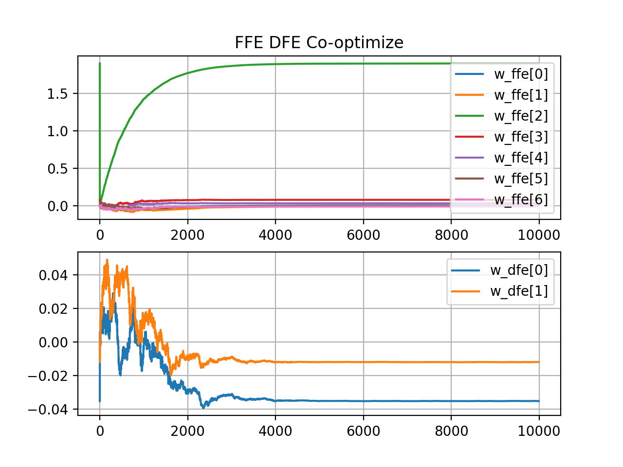
lms_equalizer performs offline adaptation and it fail due to DFE Error Propagation if reference is None

def lms_equalizer(y, mu, N, w_ffe, FFE_pre, w_dfe, voltage_levels,
        alpha=None, reference=None, update_rate=1):
    """
    voltage_levels: array
        discrete voltage levels to use in DFE optimization
    alpha: array (optional)
        used to fix the first `len(alpha)` weights in `w_dfe`, starting from the
        first pre-tap. these weights will not be optimized and will stay constant
        throughout LMS updates.
        
    reference: array (optional)
        if provided, LMS will attempt to optimize according to the error between
        the signal and reference, rather than estimating it based on the cloest
        voltage level. `len(reference)` may be less than `len(y)`, in which case
        only the first `len(reference)` updates will be optimized in this manner.
    """
    min_delay = max(FFE_post, DFE_taps)
    for k in range(min_delay, N - FFE_pre):
        y_k = y[k - FFE_post:k + FFE_pre + 1][::-1]
        z_k = z[k - DFE_taps:k][::-1]

        # alpha takes over the first len(alpha) terms of w_dfe
        if is_cooptimizing and alpha is not None:
            w_dfe[:len(alpha)] = alpha

        if w_ffe is not None:
            v_ffe[k] = np.dot(y_k, w_ffe)
        else:
            v_ffe[k] = y_k[0]

        if w_dfe is not None:
            v_dfe[k] = v_ffe[k] - np.dot(z_k, w_dfe)
        else:
            v_dfe[k] = v_ffe[k]

        z[k] = _quantize(v_dfe[k], voltage_levels)
        if reference is None or k >= len(reference):
            y_ref = z[k]
        else:
            y_ref = reference[k]

        e[k] = v_dfe[k] - y_ref
        if (k - min_delay) % update_rate == 0:
            #print(k)
            if w_ffe is not None:
                w_ffe -= mu * e[k] * y_k	# y_k
            if w_dfe is not None:
                w_dfe += mu * e[k] * z_k	# z_k

def _quantize(signal, voltage_levels):
    idx = np.abs(voltage_levels - signal).argmin()
    return voltage_levels[idx]

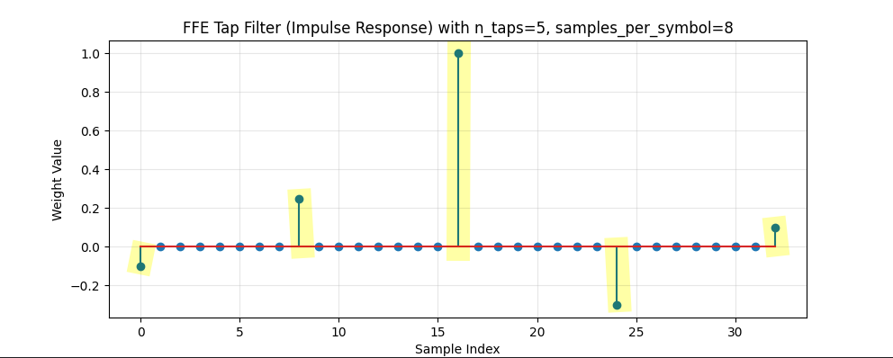
def FFE(self,tap_weights, n_taps_pre):
    """Behavioural model of FFE. Input signal is self.signal, this method modifies self.signal

    Parameters
    ----------
    tap_weights: array
        DFE tap weights

    n_taps_pre: int
        number of precursor taps
    """

    n_taps = tap_weights.size

    tap_filter = np.zeros((n_taps-1)*self.samples_per_symbol+1)

    for i in range(n_taps):
        tap_filter[i*self.samples_per_symbol] = tap_weights[i]

    length = self.signal.size
    self.signal = np.convolve(self.signal,tap_filter)
    #shift = round((n_taps_pre-n_taps)*self.samples_per_symbol)
    self.signal = self.signal[n_taps_pre*self.samples_per_symbol:n_taps_pre*self.samples_per_symbol+length]

# https://github.com/richard259/serdespy/blob/main/serdespy/receiver.py

def pam4_DFE(self, tap_weights):
    """Behavioural model of DFE for PAM-4 signal. Input signal is self.signal, this method modifies self.signal.

    Parameters
    ----------
    tap_weights: array
        DFE tap weights
    """
    
    signal_out =  np.copy(self.signal)
    n_taps = tap_weights.size
    n_symbols = int(round(self.signal.size/self.samples_per_symbol))
    half_symbol = int(round(self.samples_per_symbol/2))
    taps = np.zeros(n_taps)

    for symbol_idx in range(n_symbols-1):

        idx = symbol_idx*self.samples_per_symbol

        #decide on value of current bit 
        symbol = pam4_decision(signal_out[idx],l,m,h)

        #update taps            
        taps[1:] = taps[:-1]
        taps[0] = self.voltage_levels[symbol]

        #apply feedback to signal
        feedback = np.sum(taps*tap_weights)

        signal_out[idx+half_symbol:idx+self.samples_per_symbol+half_symbol] -= feedback

PRQSm Generator by multiplexing two PRBSn

Ilya Lyubomirsky, Finisar. PRQS Test Patterns for PAM4 [https://www.ieee802.org/3/bs/public/15_09/lyubomirsky_3bs_01_0915.pdf]

# https://github.com/richard259/serdespy/blob/main/serdespy/prs.py
# https://github.com/richard259/serdespy/blob/main/serdespy/signal.py

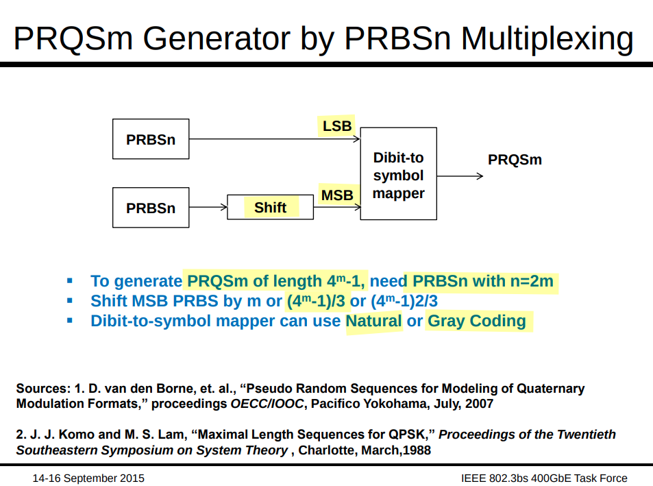
def prqs10(seed):
    """Genterates PRQS10 sequence

    Parameters
    ----------
    seed : int
        seed used to generate sequence
        should be greater than 0 and less than 2^20

    Returns
    -------
    array:
        PRQS10 sequence
    """
    
    a = prbs20(seed)
    shift = int((2**20-1)/3)
    b = np.hstack((a[shift:],a[:shift]))
    
    c = np.vstack((a,b))    # c[0,:] MSB, c[1,:] LSB

    pqrs = np.zeros(a.size,dtype = np.uint8)
    
    for i in range(a.size):
        pqrs[i] = grey_encode(c[:,i])
    
    return pqrs


def prqs12(seed):
    
    a = prbs24(seed)
    shift = int((2**24-1)/3)
    b = np.hstack((a[shift:],a[:shift]))
    
    c = np.vstack((a,b))

    pqrs = np.zeros(a.size,dtype = np.uint8)
    
    for i in range(a.size):
        if (i%1e5 == 0):
            print("i =", i)
        pqrs[i] = grey_encode(c[:,i])
    
    return pqrs

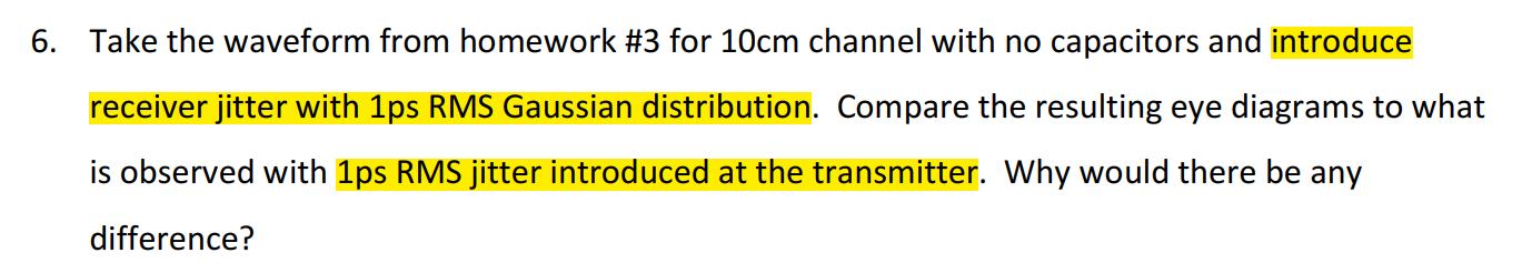
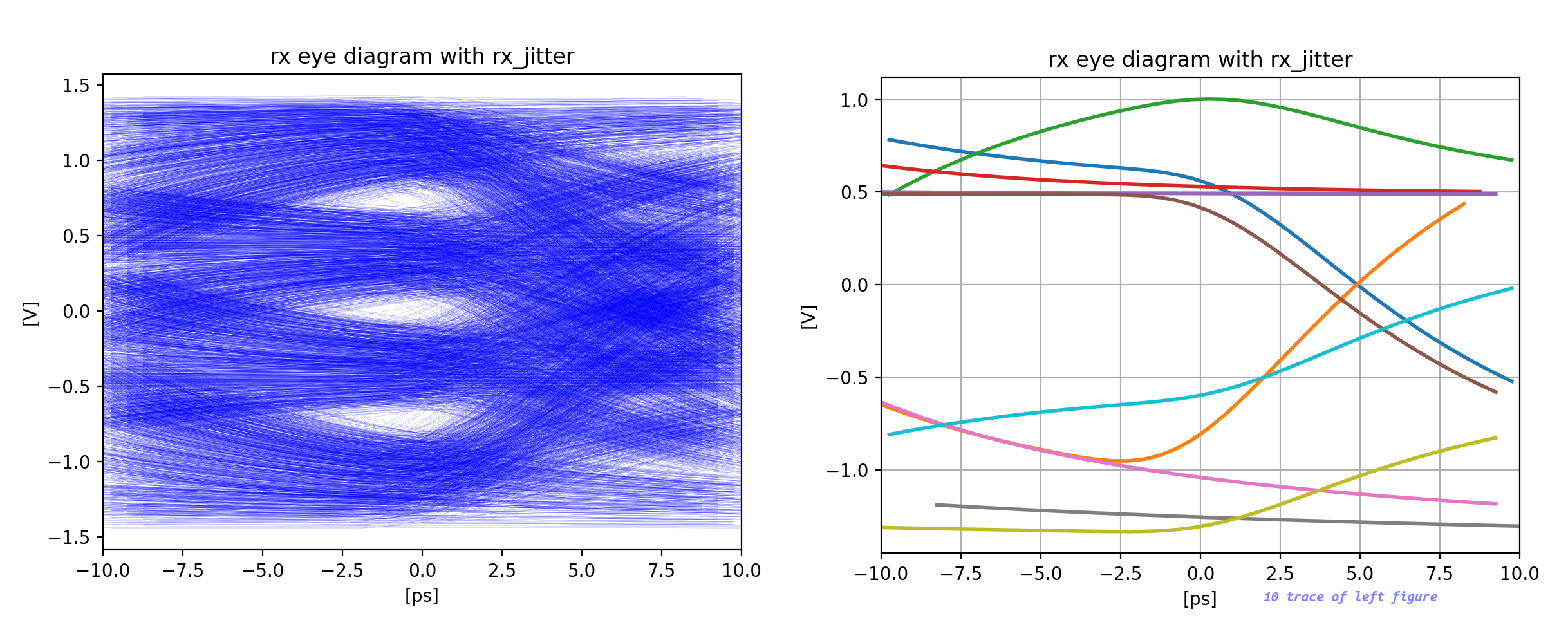
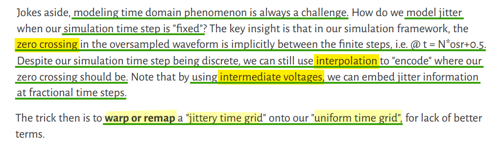
Gaussian distribution jitter

TX signal with jitter

txjitter_serdespy.drawio

The accuracy of the jitter model is constrained by the resolution defined as sample_time = UI/samples_per_symbol within the gaussian_jitter implementation.

#https://github.com/richard259/serdespy/blob/main/serdespy/transmitter.py

def gaussian_jitter(signal_ideal, UI,n_symbols,samples_per_symbol,stdev):
    """Generates the TX waveform from ideal, square, self.signal_ideal with jitter

    Parameters
    ----------
    signal_ideal: array
        ideal,square transmitter voltage waveform
    
    UI: float
        length of one unit interval in seconds
    
    n_symbols: int
        number of symbols in signal_ideal
        
    samples_per_symbol: int
        number of samples in signal_ideal corresponding to one UI
        
    stdev:
        standard deviation of gaussian jitter in seconds
    
    stdev_div_UI : float
        standard deviation of jitter distribution as a pct of UI    
    """

    #generate random Gaussian distributed TX jitter values
    epsilon = np.random.normal(0,stdev,n_symbols)
    
    epsilon.clip(UI)
    epsilon[0]=0

    #calculate time duration of each sample
    sample_time = UI/samples_per_symbol

    #initializes non_ideal (jitter) array
    non_ideal = np.zeros_like(signal_ideal)

    #populates non_ideal array to create TX jitter waveform
    for symbol_index,symbol_epsilon in enumerate(epsilon):
        epsilon_duration = int(round(symbol_epsilon/sample_time))
        start = int(symbol_index*samples_per_symbol)
        end = int(start+epsilon_duration)
        flip=1
        if symbol_index==0:
            continue
        if symbol_epsilon<0:
            start,end=end,start
            flip=-1
        non_ideal[start:end]=flip*(signal_ideal[symbol_index*samples_per_symbol-samples_per_symbol]-signal_ideal[symbol_index*samples_per_symbol])
    
    #calculate TX output waveform
    signal = np.copy(signal_ideal+non_ideal)
    return signal

RX eye_diagram with jitter by horizontal shift

Each trace is shifted by its corresponding \(\epsilon\), which is only used for visualization rather than as an input for the subsequent block.

def rx_jitter_eye(signal, window_len, ntraces, n_symbols, tstep, title,  stdev, res=600, linewidth=0.15,):
    """Genterates eye diagram with jitter introduved by splitting traces and applying 
    horizontal shift with gaussian distribution
    """
    for symbol_index,symbol_epsilon in enumerate(epsilon):
        epsilon_duration = int(round(symbol_epsilon/tstep))
        #t = np.linspace( -tstep * (((window_len-1))/2 + epsilon_duration ) ,tstep * (((window_len-1))/2 + epsilon_duration ), window_len)	# Stretch
        t = np.linspace(-tstep * (((window_len - 1)) / 2), tstep * (((window_len - 1)) / 2), window_len) + epsilon_duration*tstep	# shift

        plt.plot(t*1e12,np.reshape((traces[symbol_index][:]),window_len), color = 'blue', linewidth = linewidth)

RLM through nonlinearity

#convolution of impulse response with ideal signal
signal_filtered = sp.signal.fftconvolve(signal_ideal, h[:ir_length])

#optical modulator nonlinearity
def optical_nonlinearity(signal):
    return np.sin(np.pi*signal/5)

signal_optical = optical_nonlinearity(signal_filtered)

#calculate RLM
levels_optical = optical_nonlinearity(voltage_levels)

Vmin = (levels_optical[0]+levels_optical[3])/2

ES1 = (levels_optical[1]-Vmin)/(levels_optical[0]-Vmin)

ES2 = (levels_optical[2]-Vmin)/(levels_optical[3]-Vmin)

RLM = min((3*ES1),(3*ES2),(2-3*ES1),(2-3*ES2))

JLSD

Kevin Zheng, JLSD - Julia SerDes [https://github.com/kevjzheng/JLSD], [forked]

Kronecker product to create oversampled waveform

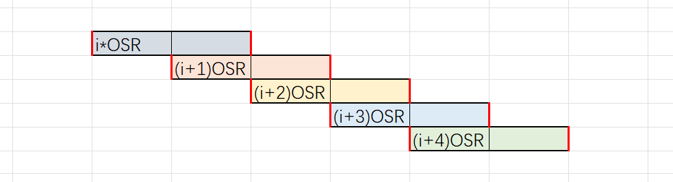
function gen_wvfm(bits; tui, osr)
	#helper function used to generate oversampled waveform
	
	Vbits = kron(bits, ones(osr)) #Kronecker product to create oversampled waveform
	dt = tui/osr
	tt = 0:dt:(length(Vbits)-1)*dt

	return tt, Vbits
end

osr.drawio

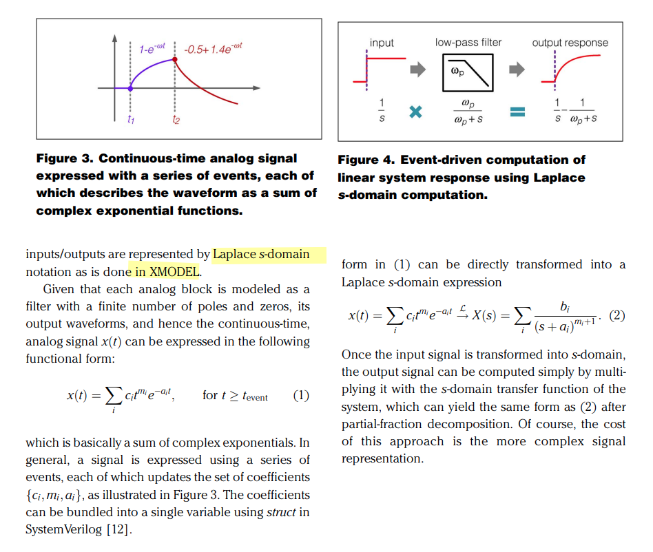
first order RC response, normalized to the time step \[ \frac{\alpha}{s+\alpha} \overset{\mathcal{L}^{-1}}{\longrightarrow} \alpha\cdot e^{-\alpha t} \]

The integral of impulse response of low pass RC filter \(\int_{0}^{+\infty} \alpha\cdot e^{-\alpha t}dt = 1\) — sum(ir*dt)

function gen_ir_rc(dt,bw,t_len)
	#helper function that directly calculates a first order RC response, normalized to the time step
    tt = [0:dt:t_len-dt;]

	#checkout the intuitive symbols!
    ω = (2*π*bw)
    ir = ω*exp.(-tt*ω)
    ir .= ir/sum(ir*dt)

    return ir
end

sum(ir)*dt = 1, i.e. the step response 1

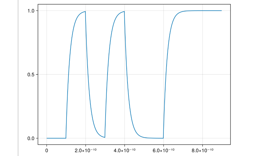
1 2	out = conv(ir, vbits)*tui/osr lines(tt, out[1:length(vbits)])

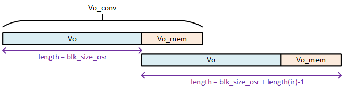
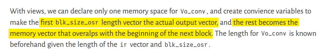
#call our convolution function; let's keep the input memory zero for now
#change the drv parameters in the struct definition to see the waveform/eye change
u_conv!(drv.Vo_conv, Vosr, drv.ir, Vi_mem=zeros(1), gain = drv.swing * param.dt);


#we will also create a non-mutating u_conv function for other uses
function u_conv(input, ir; Vi_mem = zeros(1), gain = 1)
    vconv = gain .* conv(ir, input)
    vconv[eachindex(Vi_mem)] += Vi_mem

    return vconv
end

Detailed Transmitter

tx blk diagram

Sfir_conv::Vector = zeros(param.blk_size+length(fir)-1)
Sfir = @views Sfir_conv[1:param.blk_size]
Sfir_mem = @views Sfir_conv[param.blk_size+1:end]

Vo_conv::Vector = zeros(param.blk_size_osr+lastindex(ir)-1)
Vo = @views Vo_conv[1:param.blk_size_osr]
Vo_mem = @views Vo_conv[param.blk_size_osr+1:end]

function dac_drv_top!(drv, Si)

    u_filt!(drv.Sfir_conv, Si, fir_norm, Si_mem = Sfir_mem)

    kron!(drv.Vfir, drv.Sfir, ones(osr))

    if drv.jitter_en
        drv_add_jitter!(drv, drv.Vfir)
    end

    u_conv!(drv.Vo_conv, drv.Vfir, ir, Vi_mem=Vo_mem, gain=dt*swing/2)

end

[code link]

function u_conv!(Vo_conv, input, ir; Vi_mem = Float64[], gain = 1)
    Vo_conv[eachindex(Vi_mem)] .= Vi_mem
    Vo_conv[lastindex(Vi_mem)+1:end] .= zero(Float64)

    Vo_conv .+= conv(gain .* input, ir)
    return nothing
end

TX model jitter with fixed simulation time step

warp or remap a "jittery time grid" onto our "uniform time grid"

The brilliance is that you don't need infinitesimal time steps—instead, you remap the sampling grid to account for jitter!

Vext::Vector = zeros(prev_nui*param.osr+param.blk_size_osr)	#(prev_nui + blk_size)*osr
V_prev_nui = @views Vext[end-prev_nui*param.osr+1:end]		#prev_nui*osr

Δtt_ext = zeros(param.blk_size+prev_nui+1)		# prev_nui + blk_size + 1
Δtt_prev_nui = @views Δtt_ext[end-prev_nui:end]		# prev_nui + 1

deltatt_Vext.drawio

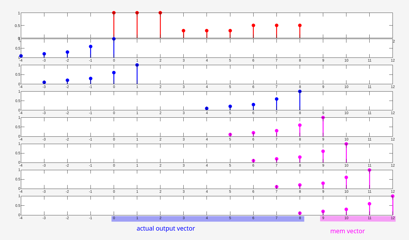
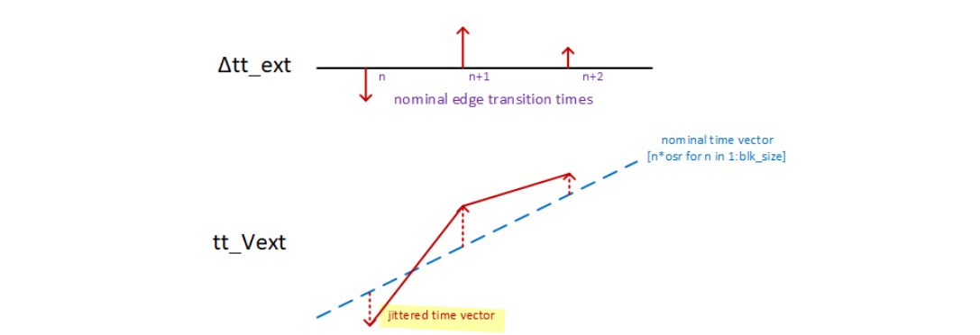
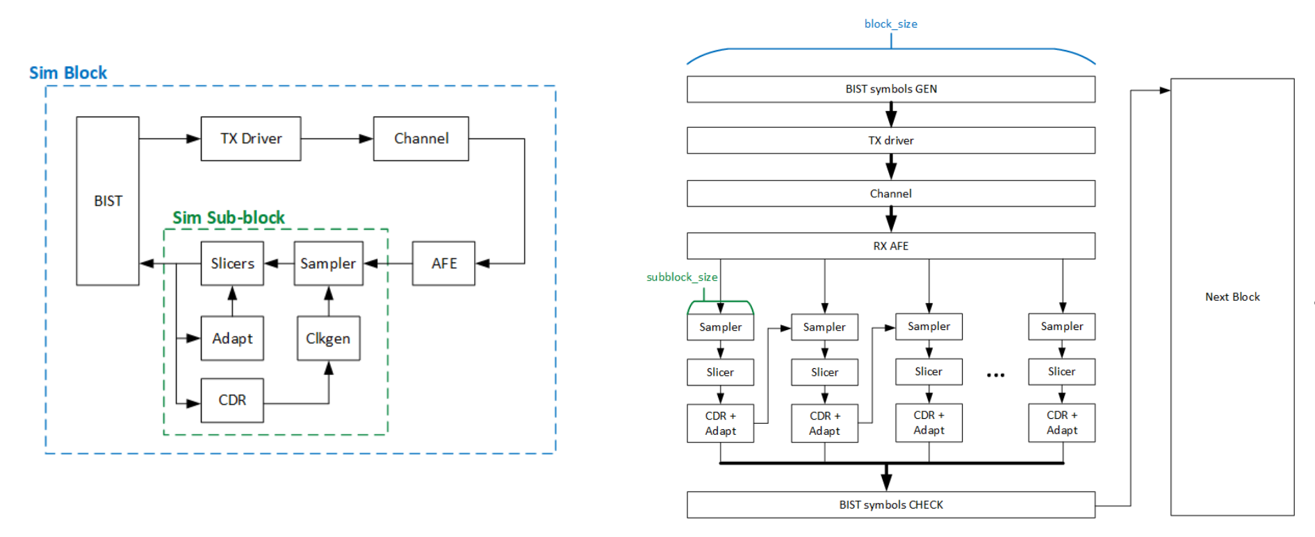
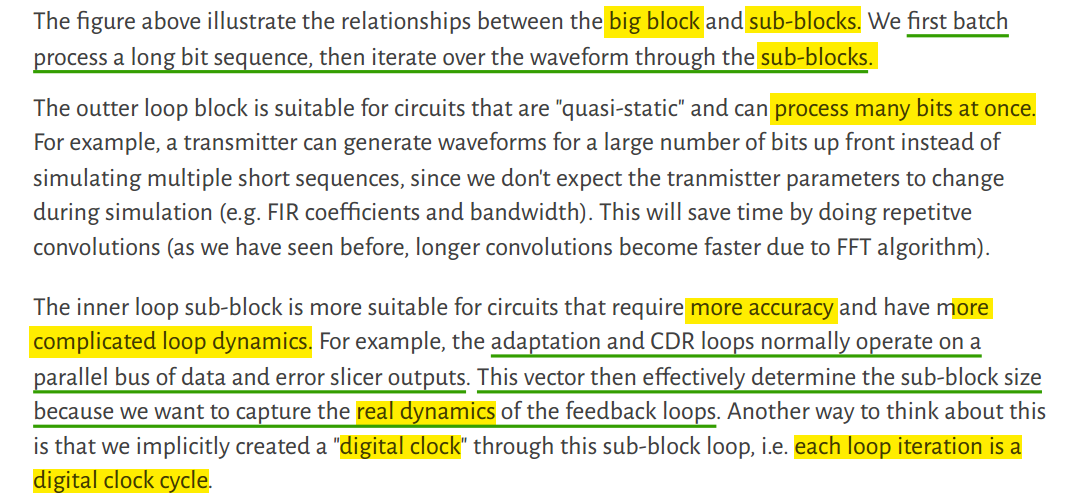
Because each symbol's width is determined by two edges, \(\Delta tt\_\text{ext}\) is is one greater than \(V_\text{ext}\)

function drv_jitter_tvec!(tt_Vext, Δtt_ext, osr)
    for n = 1:lastindex(Δtt_ext)-1
        tt_Vext[(n-1)*osr+1:n*osr] .= LinRange((n-1)*osr+Δtt_ext[n], n*osr+Δtt_ext[n+1], osr+1)[1:end-1]
    end

    return nothing
end

# tt_Vext: (prev_nui+blk_size)*osr
drv_jitter_tvec!(drv.tt_Vext, drv.Δtt_ext, param.osr);

1	itp = linear_interpolation(drv.tt_Vext, drv.Vext); #itp is a function object

itp = linear_interpolation(drv.tt_Vext, drv.Vext) create linear interpolation only, extrapolation shall not be used to avoid inducing any error

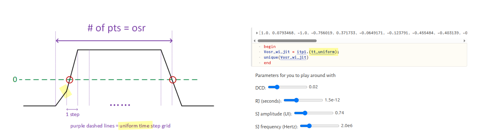
#note here tt_uniform is shifted by prev_nui/2 to give wiggle room for sampling "before" and "after" the current block. This is necessary for sinusoidal jitter
tt_uniform = (0:param.blk_size_osr-1) .+ drv.prev_nui/2*param.osr;

#To interpolate, use the itp object like a function and broadcast to a vector
Vfir = itp.(tt_uniform);

itp.drawio

tt_uniform is shifted by prev_nui/2 to give wiggle room for sampling "before" and "after" the current block. This is necessary for sinusoidal jitter

[copilot]

DCD and RJ have much smaller shifts (typically <1 UI), but SJ can oscillate over multiple UI widths, requiring this centered offset to prevent interpolation boundary errors.

function drv_jitter_tvec!(tt_Vext, Δtt_ext, osr)
    for n = 1:lastindex(Δtt_ext)-1
        # Starting from 0
        tt_Vext[(n-1)*osr+1:n*osr] .= LinRange((n-1)*osr+Δtt_ext[n], n*osr+Δtt_ext[n+1], osr+1)[1:end-1]	# drop the last
    end

    return nothing
end


# Starting from 0
tt_uniform::Vector = (0:param.blk_size_osr-1) .+ prev_nui/2*param.osr

This creates tt_Vext starting from (n-1)*osr, which means:

First segment: 0*osr + offset to 1*osr + offset = starts at 0
Second segment: 1*osr + offset to 2*osr + offset
etc.

tt_uniform must align with this same time scale for interpolation to work correctly.

Starting from 0 ensures tt_uniform aligns with the OSR sample grid and matches the time values in tt_Vext for correct interpolation.

function drv_add_jitter!(drv, Vfir)

    drv.last_sj_phi = drv_jitter_Δt!(Δtt;)

    Vext[eachindex(V_prev_nui)] .= V_prev_nui			# prev_nui*osr
    Vext[lastindex(V_prev_nui)+1:end] .= Vfir			# blk_size*osr
    Δtt_ext[eachindex(Δtt_prev_nui)] .= Δtt_prev_nui	# prev_nui + 1
    Δtt_ext[lastindex(Δtt_prev_nui)+1:end] .= Δtt		# blk_size

    drv_jitter_tvec!(tt_Vext, Δtt_ext, osr)

    drv_interp_jitter!(Vfir, tt_Vext, Vext, tt_uniform)
    return nothing
end

In each outer loop, Δtt and Vfir are created (size blk_size) and then copied into their respective extended buffers, Δtt_ext and Vext.

tx_view.drawio

tt_uniform.drawio

channel

noise_Z::Float64 = 50  # termination impedance with thermal noise
noise_dbm_hz::Float64 = -174
noise_rms::Float64 = sqrt(0.5/param.dt*10^((noise_dbm_hz-30.0)/10)*noise_Z)

ch.Vch .+= noise_rms .* randn(blk_size_osr)

\[ P_\text{n,dBm/Hz} = 10\times\log_{10} (k_B T / 10^{-3}) = 10\times\log_{10} (k_B T) + 30=-174 \]

Then, \(k_B T = 10^{\frac{-174 - 30}{10}}\)

we have

\[ \sigma_n^2 = 4\cdot k_B T \cdot R \cdot \frac{f_s}{2} = k_B T \cdot R \cdot 2f_s= \frac{\color{red}{2}}{T_s} \cdot 10^{\frac{-174 - 30}{10}} \cdot R \]

noise_rms::Float64 = sqrt(2/param.dt*10^((noise_dbm_hz-30.0)/10) rather than ~~sqrt(0.5/param.dt*10^((noise_dbm_hz-30.0)/10)~~

Clkgen-PI

@kwdef mutable struct Clkgen

    nphases::Int8

    pi_res = 8
    pi_max_code = 2^pi_res-1
    pi_ui_cover = 4
    pi_codes_per_ui = 2^pi_res/pi_ui_cover
    pi_nonlin_lut = zeros(2^pi_res) #introduce INL here
    pi_code_prev = 0
    pi_wrap_ui = 0
    pi_wrap_ui_Δcode = pi_max_code-10

end

Parameter	Default	Meaning
`pi_res`	`8`	PI has 8-bit resolution
`pi_max_code`	`2^8 - 1 = 255`	Code range is 0–255
`pi_ui_cover`	`4`	The full 256 codes span 4 UI
`pi_codes_per_ui`	`2^8 / 4 = 64`	64 codes per UI
`pi_wrap_ui_Δcode`	`255 - 10 = 245`	Wrap detection threshold
`pi_wrap_ui`	`0`	Starts with zero wraps
`pi_code_prev`	`0`	Previous PI code starts at 0

The margin of 10 (pi_max_code - 10) ensures that even if the CDR makes a moderately large step (up to ±10 codes), it won't be mistaken for a wrap. This is safe as long as the CDR loop bandwidth is low enough that per-update code changes stay well below 10

function clkgen_pi_itp_top!(clkgen; pi_code)

    Δpi_code = pi_code-pi_code_prev
    if abs(Δpi_code) > pi_wrap_ui_Δcode
        pi_wrap_ui -= sign(Δpi_code)*pi_ui_cover
    end

    Φ0 = osr*(pi_wrap_ui + (pi_code + pi_nonlin_lut[pi_code+1])/pi_codes_per_ui)
    Φstart = (cur_subblk-1)*subblk_size*osr
    Φnom = Φstart:osr:Φstart+(subblk_size-1)*osr
    Φskew = kron(ones(Int(subblk_size/nphases)), skews/tui*osr)
    Φrj = rj/tui*osr*randn(subblk_size)

    @. clkgen.Φo_subblk = Φ0 + Φnom + Φskew + Φrj

end

How Wrap Detection Works

PI code:   0 ---------> 255 | 0 ---------> 255 | 0 ---> ...
           ╰── 4 UI ──╯     ╰── 4 UI ──╯

Example wrap-forward:  pi_code: 253 → 2  (Δ = -251, |Δ| > 245)
  → pi_wrap_ui += pi_ui_cover (+4 UI)

Example wrap-backward: pi_code: 2 → 253  (Δ = +251, |Δ| > 245)
  → pi_wrap_ui -= pi_ui_cover (-4 UI)

Variable	Role
`pi_wrap_ui`	Accumulated wrap count in UI — keeps `Φ0` continuous across wraps
`Φ0`	PI-controlled phase offset (CDR tracking loop output)

function cdr_top!(cdr, Sd, Se)

    for n = findall(eslc_nvec.!=0)
        if Sd_val[n:n+2] in filt_patterns
            vote = sign(Se[n][1].-0.5)*sign(Sd_val[n]-Sd_val[n+2])
            ki_accum += ki*vote
            pd_accum += pd_gain*(kp*vote + ki_accum)
        end
    end

    cdr.pd_accum = (pd_accum < 0) ? pi_bnd + pd_accum : (pd_accum >= pi_bnd) ? pd_accum - pi_bnd : pd_accum
    cdr.pi_code = Int(floor(cdr.pd_accum))

end

Wraps pd_accum into [0, pi_bnd) (i.e., [0, 256) for 8-bit PI), then floors it to produce the integer pi_code that feeds back to clkgen_pi_itp_top!. This is the modular accumulator — the same wrapping that pi_wrap_ui in the clock generator unwraps.

sampler

@kwdef mutable struct Splr
    ir::Vector{Float64}

    Vo_conv::Vector = zeros(param.blk_size_osr+lastindex(ir)-1)
    Vo = @views Vo_conv[1:param.blk_size_osr]
    Vo_mem = @views Vo_conv[param.blk_size_osr+1:end]

    prev_nui = 16
    Vext::Vector = zeros(prev_nui*param.osr+param.blk_size_osr)
    V_prev_nui = @views Vext[end-prev_nui*param.osr+1:end]

	# tt_Vext is constant
    tt_Vext = -prev_nui/2*param.osr:length(Vext)-prev_nui/2*param.osr-1
	itp_Vext = nothing

    So = CircularBuffer{Float64}(param.blk_size)
    So_subblk::Vector = zeros(param.subblk_size)
end

adaptation and CDR loop

## pseudo-code

## outter loop block 
run_blk_iter(trx, ++0, nblk, sim_blk) begin
    pam_gen_top!(bist)
    dac_drv_top!(drv, bist.So)
    ch_top!(ch, drv.Vo)
    sample_itp_top!(splr, ch.Vo)	# update splr.Vext, splr.itp_Vext
    
    ## inner loop sub-blok
    run_blk_iter(trx, ++0, nsubblk, sim_subblk) begin
       	clkgen_pi_itp_top!(clkgen, pi_code=cdr.pi_code)
        sample_phi_top!(splr, clkgen.Φo_subblk)
        # dslc.So[1:subblk_size]
        slicers_top!(dslc, splr.So_subblk, ref_code=[[128],[128],[128],[128]])
        # eslc.So[1:subblk_size]
        slicers_top!(eslc, splr.So_subblk, ref_code=adpt.eslc_ref_vec)
        cdr_top!(cdr, dslc.So, eslc.So)
        adpt_top!(adpt, dslc.So, eslc.So)
        
        append!(bist.Si, [sum(dvec) for dvec in dslc.So])
        push!(wvfm.buffer12, adpt.eslc_ref_code)
        push!(wvfm.buffer22, cdr.pi_code)
    end
    
    ber_checker_top!(bist)
    append!(wvfm.buffer11, drv.Vo)
    append!(wvfm.buffer21, ch.Vo)
    append!(wvfm.buffer31, splr.So)
    append!(wvfm.eye1.buffer, splr.Vo)
    wvfm.eslc_ref_ob.val = adpt.eslc_ref_code*eslc.dac_lsb+eslc.dac_min
end

clkgen = TrxStruct.Clkgen(nphases = 4, skews = [0e-12, 0e-12, 0e-12, 0e-12])
dslc = TrxStruct.Slicers(N_per_phi = ones(UInt8, clkgen.nphases), dac_min = -0.1, dac_max = 0.1)
eslc = TrxStruct.Slicers(N_per_phi = UInt8.([1,0,0,0]),dac_min = 0, dac_max = 0.5)
cdr = TrxStruct.Cdr(Neslc_per_phi = eslc.N_per_phi)
adpt = TrxStruct.Adpt(Neslc_per_phi = eslc.N_per_phi

@kwdef mutable struct Splr
    # continuous signal
    Vo_conv::Vector = zeros(param.blk_size_osr+lastindex(ir)-1)
    Vo = @views Vo_conv[1:param.blk_size_osr]
    Vo_mem = @views Vo_conv[param.blk_size_osr+1:end]
    ...
    # sampled signal
    So = CircularBuffer{Float64}(param.blk_size)
    So_subblk::Vector = zeros(param.subblk_size)
    itp_Vext = nothing
end


function sample_itp_top!(splr, Vi)
    u_conv!(Vo_conv, Vi, ir, Vi_mem=Vo_mem, gain=dt)
    splr.itp_Vext = linear_interpolation(tt_Vext, Vext)
end


function clkgen_pi_itp_top!(clkgen; pi_code)
    Φskew = kron(ones(Int(subblk_size/nphases)), skews/tui*osr)
    Φrj = rj/tui*osr*randn(subblk_size)
    ...
    @. clkgen.Φo_subblk = Φ0 + Φnom + Φskew + Φrj	# subblk_size
    append!(clkgen.Φo, clkgen.Φo_subblk)
end


function sample_phi_top!(splr, Φi)
    splr.So_subblk .= itp_Vext.(Φi)		# subblk_size
    append!(splr.So, splr.So_subblk)
end


@kwdef mutable struct Cdr
    Neslc_per_phi::Vector
    nphases = length(Neslc_per_phi)
    Sd_prev = 0

    # [1,0,0,0, 1,0,0,0, 1,0,0,0,...], subblk_size-elements repeating [1,0,0,0]
    eslc_nvec = kron(ones(Int(param.subblk_size/nphases)),Neslc_per_phi)

    filt_patterns = [[0, 1, 1], [1, 1, 0]]
end


@kwdef mutable struct Adpt
    Neslc_per_phi::Vector
    nphases = length(Neslc_per_phi)
    Sd_prev = 0

    eslc_ref_accum = 128.0
    eslc_ref_max = 255
    eslc_ref_code = floor(eslc_ref_accum)

    # [1,0,0,0, 1,0,0,0, 1,0,0,0,...], subblk_size-elements repeating [1,0,0,0]
    eslc_nvec = kron(ones(Int(param.subblk_size/nphases)),Neslc_per_phi)

    eslc_filt_patterns = [[0, 1, 1], [1, 1, 0]]

    # [[eslc_ref_code], [], []. []]
    eslc_ref_vec = [eslc_ref_code*ones(Int,n) for n in Neslc_per_phi]
end

Sign-Sign Mueller-Muller CDR - cdr_top!

pattern	main cursor	Se (assuming \(h_0=\operatorname{dLev}\))	vote
011	\(s_{011}=-h_1+h_0+h_{-1}\)	\(\operatorname{sign}({-h_1+h_{-1}})\)	\(\operatorname{sign}({h_1-h_{-1}})\)
110	\(s_{110}=h_1+h_0-h_{-1}\)	\(\operatorname{sign}({h_1-h_{-1}})\)	\(\operatorname{sign}({h_1-h_{-1}})\)

function cdr_top!(cdr, Sd, Se)
    pi_bnd = 2^pi_res
    Sd_val = [Sd_prev; [sum(dvec) for dvec in Sd]]

    for n = findall(eslc_nvec.!=0)
        if Sd_val[n:n+2] in filt_patterns
            vote = sign(Se[n][1].-0.5)*sign(Sd_val[n]-Sd_val[n+2])
            ki_accum += ki*vote
            pd_accum += pd_gain*(kp*vote + ki_accum)
        end
    end

    cdr.Sd_prev = Sd_val[end]
end

cdr_adapt.drawio

\(\operatorname{dLev}\) adaptation \[ dLev_{n+1} = dLev_n + \mu\cdot \operatorname{sign}( e_n) \]

function adpt_top!(adpt, Sd, Se)
    Sd_val = [Sd_prev; [sum(dvec) for dvec in Sd]]

    ref_accum = adpt.eslc_ref_accum

    for n = findall(eslc_nvec.!=0)
        ref_accum +=  (Sd_val[n:n+2] in eslc_filt_patterns) ?
                        mu_eslc*sign(Se[n][1].-0.5) : 0
    end
    adpt.eslc_ref_accum =   ref_accum < 0 ? 0 :
                            ref_accum > eslc_ref_max ? eslc_ref_max :
                            ref_accum
    adpt.eslc_ref_code = floor(adpt.eslc_ref_accum)
    adpt.eslc_ref_vec = [adpt.eslc_ref_code*ones(Int,n) for n in Neslc_per_phi]

    adpt.Sd_prev = Sd_val[end]
end

dslc.So & eslc.So initialization with Number of comparisons executed during each phase N_per_phi

@kwdef mutable struct Slicers
    N_per_phi::Vector
    nphases = length(N_per_phi)
    dac_res = 8
    dac_min = 0
    dac_max = 0.5
    dac_lsb = (dac_max-dac_min)/2^dac_res

    So = [zeros(Bool, Int(N_per_phi[n%nphases+1])) for n in 0:param.subblk_size-1]
end


function slicers_top!(slc, Si; ref_code)
    ref_lvl = [(dac_min .+ dac_lsb * ref_code[n]) for n in 1:nphases]

    for n = eachindex(Si)
        phi_idx = (n-1)%nphases + 1
        nslc = N_per_phi[phi_idx]
        if nslc != 0
            slc.So[n] .=  (ref_lvl[phi_idx]
                            + ofsts[phi_idx]
                            + (noise_rms * randn(nslc))		# noise per comparison
                            ) .< Si[n]

        end
    end
end

For DSLC: N_per_phi=[1,1,1,1]

dslc.So = [zeros(Bool, Int(N_per_phi[n%nphases+1])) for n in 0:param.subblk_size-1]
          = [zeros(Bool, 1), zeros(Bool, 1), zeros(Bool, 1), zeros(Bool, 1),
             zeros(Bool, 1), zeros(Bool, 1), ...]
          = [[false], [false], [false], [false], 
             [false], [false], ...]

For ESLC: N_per_phi=[1,0,0,0]

eslc.So = [zeros(Bool, Int(N_per_phi[n%nphases+1])) for n in 0:param.subblk_size-1]

n     │ n%4+1 │ N_per_phi[n%4+1] │ zeros(Bool, ...)
──────┼───────┼──────────────────┼──────────────────
0     │ 1     │ 1                │ [false] (1 bool)
1     │ 2     │ 0                │ [] (0 bools - EMPTY!)
2     │ 3     │ 0                │ [] (0 bools - EMPTY!)
3     │ 4     │ 0                │ [] (0 bools - EMPTY!)
4     │ 1     │ 1                │ [false] (1 bool)
5     │ 2     │ 0                │ [] (EMPTY!)
...

elastic buffer to model frequency offsets of TRX

TODO 📅

TX Fixed block size
RX sub-block keep symbol count fixed but let sample-time span vary
dynamic sub-block count

A sub-block should usually consume a fixed number of RX symbols because the downstream RX logic is organized around symbol-domain operations

f_rx = f_tx * (1 + ppm)

RX sample spacing in TX-grid units osr_rx = osr_tx / (1 + ppm)

Sam Palermo's

continuous time filter (channel, ctle); impulse response

digital filter (FFE, DFE): repmat by samples per UI

Sam Palermo. ECEN 720: High-Speed Links Circuits and Systems [https://people.engr.tamu.edu/spalermo/ecen720.html]

repmat

>> repmat([1,2,3], 3, 1)

ans =

     1     2     3
     1     2     3
     1     2     3

>> reshape(repmat([1,2,3], 3, 1), 1, 3*3)

ans =

     1     1     1     2     2     2     3     3     3

Generating an Impulse Response from S-Parameters

ECEN720: High-Speed Links Circuits and Systems Spring 2025 [https://people.engr.tamu.edu/spalermo/ecen689/lecture3_ee720_tdr_spar.pdf]

spline: Cubic spline data interpolation

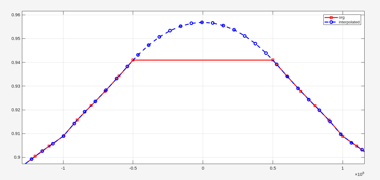
Hm_ds_interp=spline(fds_m,Hm_ds,f_ds_interp); % Interpolate for FFT point number
figure(Name='spline function')
plot(fds_m, Hm_ds, '-rs', LineWidth=2)
hold on
plot(f_ds_interp, Hm_ds_interp, '--bo', LineWidth=2)
legend('org', 'interpolated'); grid on

impulse response from ifft of interpolated frequency response

% https://people.engr.tamu.edu/spalermo/ecen689/xfr_fn_to_imp.m

% Generate Random Data
nt=1e3;         %number of bits
m=rand(1,nt+1);     %random numbers between 1 and zero, will be quantized later
m=-1*sign(m-0.5).^2+sign(m-0.5)+1;


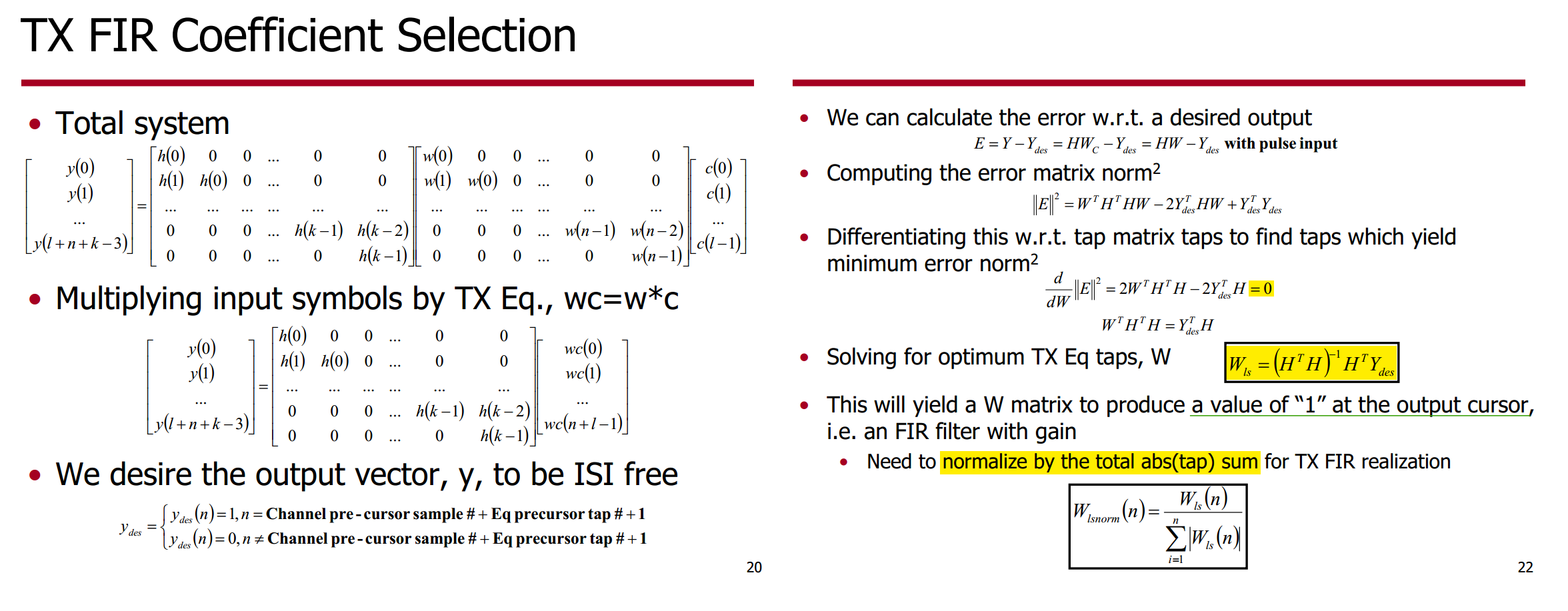
% TX FIR Equalization Taps
eq_taps=[1];
m_fir=filter(eq_taps,1,m);


m_dr=reshape(repmat(m_fir,bit_period,1),1,bit_period*size(m_fir,2));

data_channel=0.5*conv(sig_ir(:,1),m_dr(1:nt*bit_period));

subplot(3,1,1)

FileName = './peters_01_0605_B12_thru.s4p';
SingleEndedData = read(rfdata.data, FileName);
Freq = SingleEndedData.Freq;
DifferentialSparams = s2sdd(SingleEndedData.S_Parameters);
rfdata.network('Data', DifferentialSparams, 'Freq', Freq);
H21 = DifferentialSparams(2,1,:);

plot(Freq'*1e-9, abs(H21(:)),'-r', LineWidth=2);
xlabel('GHz'); ylabel('Mag(H21)'); grid on;


subplot(3,1,2)
load './ir_B12.mat';
tsample=1e-12;  % Impluse response has 1ps time step
sample_num=size(ir,1);  
sig_ir=ir(:,1); 

time=(1:size(sig_ir,1))*1e-12;

plot(time, sig_ir, '-b', LineWidth=2);
title('Channel Impulse Response (sig_ir)'); grid on;


subplot(3,1,3)
step_resp = cumsum(sig_ir); % Ts factor embedded in sig_ir
plot(time, step_resp, '-m', LineWidth=2);
title('Channel Step Response (cumsum(sig_ir)'); grid on;

1 2	plot(ch1_freqs,20log10(abs(ch1)),'-b',Freq'1e-9,20*log10(abs(H21)),'-r'); legend('From Impulse Response','Measured');

plot eye diagram

% https://people.engr.tamu.edu/spalermo/ecen689/channel_data.m

data_channel=0.5*conv(sig_ir(:,1),m_dr(1:nt*bit_period));

j=1;
offset=144;

for ( i=55:floor(size(data_channel,2) / bit_period)-500)
    eye_data(:,j) = 2*data_channel(floor((bit_period*(i-1)))+offset: floor((bit_period*(i+1)))+offset);
    j=j+1;
end

time=0:2*bit_period;
plot(time,eye_data);

If your 2D array represents multiple data series (e.g., each column is a separate line series sharing the same x-axis values), the plot() function is the most straightforward method.

[https://people.engr.tamu.edu/spalermo/ecen689/lecture4_ee720_channel_pulse_model.pdf]

% https://people.engr.tamu.edu/spalermo/ecen689/tx_eq.m

precursor_samples=10;
pulse_response=conv(ir_process,ones(1,bit_period));
[max_pulse_value,max_pulse_time]=max(pulse_response);
sample_times=[max_pulse_time-1*precursor_samples*bit_period:bit_period:max_pulse_time+30*bit_period];
sample_values=pulse_response(sample_times);

% Construct H matrix
H(:,1)=sample_values';
H(size(sample_values,1)+1:size(sample_values,1)+eq_tap_number-1,1)=0;
for i=2:eq_tap_number
    H(1:i-1,i)=0;
    H(i:size(sample_values,1)+i-1,i)=sample_values';
    H(size(sample_values,1)+i:size(sample_values,1)+eq_tap_number-1,1)=0;
end;


% Construct Y matrix
Ydes(1:precursor_samples+precursor_number,1)=0;
Ydes(precursor_samples+precursor_number+1,1)=1;
Ydes(precursor_samples+precursor_number+2:size(H,1),1)=0;

W=(H'*H)^(-1)*H'*Ydes

Itot=1;
taps=Itot*W/sum(abs(W));

TX FIR Tap Resolution

% https://people.engr.tamu.edu/spalermo/ecen689/tx_eq.m

taps_abs=abs(taps);
taps_sign=sign(taps);

partition=[1/(2*(2^num_bits-1)):1/(2^num_bits-1):1-1/(2*(2^num_bits-1))];
codebook=[0:1/(2^num_bits-1):1];
[index,abs_taps_quan]=quantiz(abs(taps),partition,codebook);
taps_quan=taps_sign'.*abs_taps_quan;
taps_quan(precursor_number+1)=sign(taps_quan(precursor_number+1))*(1-(sum(abs(taps_quan))-abs(taps_quan(precursor_number+1))));

CTLE modeling by impulse response

Given two impulse response \(h_0(t)\), \(h_1(t)\) and \(h_0(t)*h_1(t) = h_{tot}(t)\), we have \[ T_s h_0(kT_s) * T_sh_1(kT_s) = T_s h_{tot}(kT_s) \]

To use the filter function with the b coefficients from an FIR filter, use y = filter(b,1,x)

CTLE response from frequency response using ifft

data-driven frequency table

% https://people.engr.tamu.edu/spalermo/ecen689/gen_ctle.m

Hk_ext = [Hk conj(Hk(end-1:-1:2))] ;

hn_ext_ifft = real(ifft(Hk_ext, 'symmetric'));
hn_ext_ifft(1) = (2 * hn_ext_ifft(1));
%interpolate ifft
N = length(ctle.f_arr);
Ts = (1 / (2*fmax));
t_arr = ((0 : (N-1)) * Ts); Tmax = t_arr(end); %10e-9; 
treqd = (0 : time_step : Tmax);
%interpolate step response instead of impulse response
sr_ifft = cumsum(hn_ext_ifft(1:length(t_arr))); sr_ifft_t = t_arr;
sr_interp = interp1(sr_ifft_t, sr_ifft, treqd, 'spline');
ir_interp = diff(sr_interp);
ir_ctle = ir_interp; clear ir_interp;

%scale by gain adjustment factor
ir_ctle = (ir_ctle * ctle.gain_adjust_fac);
ir_out = filter(ir_ctle, 1, ir_in);

CTLE response from pole/zero using tf & impulse

1
2
3

H21 = tf();
tsamples = 0:Ts:nUI
ir = Ts*impulse(H21, tsamples)  % scaling by Ts is necessary

CTLE response from pole/zero using bilinear discretization

analytical pole/zero transfer function, [Google AI Mode]

% https://people.engr.tamu.edu/spalermo/ecen689/gen_ctle.m

A_dc=max(A_dc,1e-3);
zeq=max(zeq,1);
peq=max(peq,1);

gbw_rad=gbw*2*pi;
zeq_rad=zeq*2*pi;
peq_rad=peq*2*pi;

ppar=(gbw_rad*zeq_rad)/(A_dc*peq_rad);

a_tf=A_dc*peq_rad*ppar;
b_tf=A_dc*peq_rad*ppar*zeq_rad;
c_tf=zeq_rad;
d_tf=(peq_rad+ppar)*zeq_rad;
e_tf=peq_rad*ppar*zeq_rad;


B_filt=[2*a_tf/time_step+b_tf;
    2*b_tf;
    b_tf-2*a_tf/time_step]';

A_filt=[4*c_tf/time_step^2+2*d_tf/time_step+e_tf;
    2*e_tf-8*c_tf/time_step^2;
    4*c_tf/time_step^2-2*d_tf/time_step+e_tf]';

B_filt=B_filt/A_filt(1);
A_filt=A_filt/A_filt(1);

ir_out=filter(B_filt,A_filt,ir_in);

rx dfe

pseudo linear equalizer

% https://people.engr.tamu.edu/spalermo/ecen689/channel_data_pulse_pda_dfe.m

% Take 10 pre-cursor, cursor, and 90 post-cursor samples
sample_offset=opt_sample*bit_period;
for i=1:101
sample_points(i)=max_data_ch_idx+sample_offset+(i-11)*bit_period;
end
sample_values=data_channel(sample_points);
sample_points=(sample_points-max_data_ch_idx)./bit_period;

channel_delay=max_data_ch_idx-(20*bit_period+1);  % !! 20*bit_period = 2000

% Include DFE Equalization
dfe_tap_num=2;
dfe_taps(1:dfe_tap_num)=sample_values(12:12+dfe_tap_num-1);  % h1, h2...

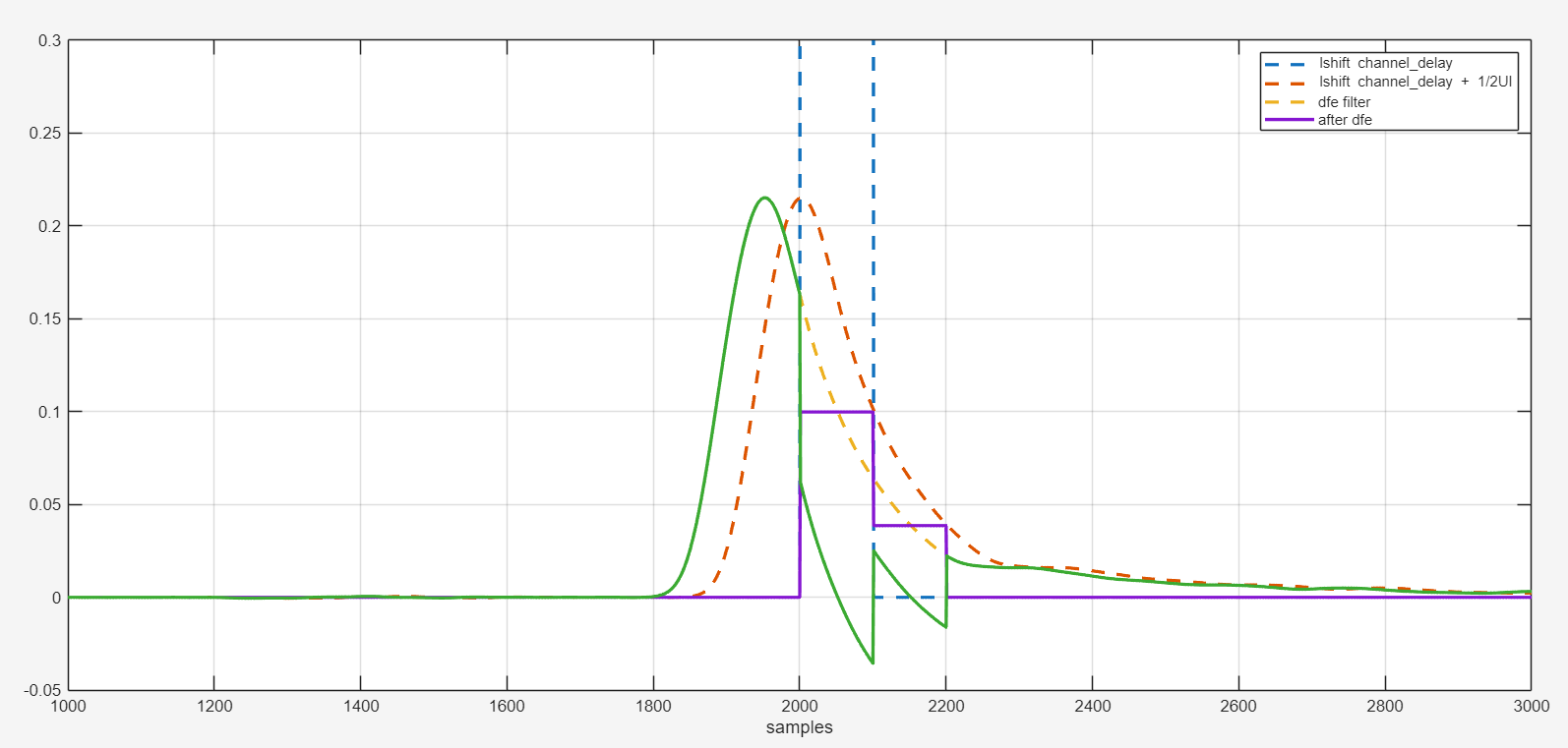
% Note this isn't a strtict DFE implementation - as I am not making a
% decision on the incoming data.  Rather, I am just using the known data
% that I transmitted, delay matching this with the channel data, and using 
% it to subtract the ISI after weighting with the tap values.  But, I think 
% it is good enough for these simulations.
m_dfe=filter(dfe_taps,1,m);
m_dfe_dr=reshape(repmat(m_dfe,bit_period,1),1,bit_period*size(m_dfe,2));

data_channel=data_channel';
dfe_fb_offset=floor(bit_period/2); % Point at which the DFE taps are subtracted - can be anything from 0 to UI-1*time_step
data_channel_dfe=data_channel(channel_delay+dfe_fb_offset:channel_delay+dfe_fb_offset+size(m_dfe_dr,2)-1)-m_dfe_dr;

plot(m_dr, '--', LineWidth=2); hold on
plot(data_channel(channel_delay:end), '--', LineWidth=2)
hold on
plot(data_channel(channel_delay+dfe_fb_offset:channel_delay+dfe_fb_offset+size(m_dfe_dr,2)-1), '--', LineWidth=2)
plot(m_dfe_dr, LineWidth=2); plot(data_channel_dfe, LineWidth=2)
xlim([1000, 3000]); ylim([-0.05, 0.3]); xlabel('samples'); grid on
legend('lshift channel\_delay', 'lshift channel\_delay + 1/2UI', 'dfe filter', 'after dfe')

SerDesSystemCProject

Lewis Liu [https://github.com/LewisLiuLiuLiu/SerDesSystemCProject]

sasasatori, SystemC简介与安装 [https://www.cnblogs.com/sasasatori/p/17865550.html]

Rahul Bhadani. [SystemC-AMS Quick Installation Guide] [SystemC Quick Installation Guide]

SerDes - High-Speed Serial Link Simulator (SystemC-AMS)

Install SystemC

## CMakeLists.txt

set (CMAKE_CXX_STANDARD 11 CACHE STRING
"C++ standard to build all targets. Supported values are 98, 11, 14, and 17.")

test systemc

cmake_minimum_required(VERSION 3.0)
project(test_systemc)

list(APPEND CMAKE_PREFIX_PATH ${SYSTEMC_HOME})  
find_package(SystemCLanguage CONFIG REQUIRED)
set (CMAKE_CXX_STANDARD ${SystemC_CXX_STANDARD})


add_executable(test_systemc main.cxx)
target_link_libraries(test_systemc SystemC::systemc)

Install SystemC-AMS

1
2
3

mkdir build && cd build
../configure CXXFLAGS="-std=c++14" --prefix=/home/software/systemc-ams-2.3.4 --with-systemc=/home/software/systemc-2.3.4  --disable-systemc_compile_check
make install

DaVE

Byongchan Lim. DaVE — tools regarding on analog modeling, validation, and generation, [https://github.com/StanfordVLSI/DaVE]

TODO 📅

Statistical Eye

Sanders, Anthony, Michael Resso and John D'Ambrosia. “Channel Compliance Testing Utilizing Novel Statistical Eye Methodology.” (2004) [https://people.engr.tamu.edu/spalermo/ecen689/stateye_theory_sanders_designcon_2004.pdf]

X. Chu, W. Guo, J. Wang, F. Wu, Y. Luo and Y. Li, "Fast and Accurate Estimation of Statistical Eye Diagram for Nonlinear High-Speed Links," in IEEE Transactions on Very Large Scale Integration (VLSI) Systems, vol. 29, no. 7, pp. 1370-1378, July 2021 [https://sci-hub.se/10.1109/TVLSI.2021.3082208]

HSPICE® User Guide: Signal Integrity Modeling and Analysis, Version Q-2020.03, March 2020

IA Title: Common Electrical I/O (CEI) - Electrical and Jitter Interoperability agreements for 6G+ bps, 11G+ bps, 25G+ bps I/O and 56G+ bps IA # OIF-CEI-04.0 December 29, 2017 [pdf]

J. Park and D. Kim, "Statistical Eye Diagrams for High-Speed Interconnects of Packages: A Review," in IEEE Access, vol. 12, pp. 22880-22891, 2024 [pdf]

StatOpt

Savo Bajic, ECE1392, Integrated Circuits for Digital Communications: StatOpt in Python [https://savobajic.ca/projects/academic/statopt] [https://www.eecg.utoronto.ca/~ali/statopt/main.html]

TODO 📅

pystateye

Chris Li. pystateye - A Python Implementation of Statistical Eye Analysis and Visualization [https://github.com/ChrisZonghaoLi/pystateye]

TODO 📅

other framework

pyBERT

David Banas. pyBERT: Free software for signal-integrity analysis [https://github.com/capn-freako/PyBERT], [intro]

—. Free yourself from IBIS-AMI models with PyBERT [https://www.edn.com/free-yourself-from-ibis-ami-models-with-pybert/]

TODO 📅

PyChOpMarg

David Banas. Python implementation of COM, as per IEEE 802.3-22 Annex 93A. [https://github.com/capn-freako/PyChOpMarg]

CC Chen. Why Channel Operating Margin? [https://youtu.be/mrXur-WbrR8]

TODO 📅

mmse_dfe

Chris Li, jointly optimizing feed-forward equalizer (FFE) and decision-feedback equalizer (DFE) tap weights [https://github.com/ChrisZonghaoLi/mmse_dfe]

John M. Cioffi, Chapter 3 - Equalization [https://cioffi-group.stanford.edu/doc/book/chap3.pdf]

TODO 📅

ngscopeclient

[https://github.com/ngscopeclient/scopehal-apps]

TODO 📅

SignalIntegrity

SignalIntegrity: Signal and Power Integrity Tools [https://github.com/Nubis-Communications/SignalIntegrity]

TODO 📅

Helper Functions

int2bits

[https://github.com/kevjzheng/JLSD/blob/4ac92476b67ce78e01820502eb3b4afb6d31bcd7/src/blks/BlkBIST.jl#L126-L128]

1
2
3

function int2bits(num, nbit)
	return [Bool((num>>k)%2) for k in nbit-1:-1:0]
end

generate PAM symbols

here Big Endian

#generate PAM symbols
   fill!(So, zero(Float64)) #reset So to all 0
   for n = 1:bits_per_sym
       @. So = So + 2^(bits_per_sym-n)*So_bits[n:bits_per_sym:end]
   end

function int2bits(num, nbit)
    return [Bool((num>>k)%2) for k in nbit-1:-1:0]
end


 Si_bits .= vec(stack(int2bits.(Si, bits_per_sym)))

eye diagram based on `heatmap`

function w_gen_eye_simple_test(input,x_npts_ui, x_npts, y_range, y_npts; osr, x_ofst=0)
    heatmap = zeros(x_npts, y_npts)

    input_x = 0:1/osr:(lastindex(input)-1)/osr
    itp_resample = linear_interpolation(input_x, input) # interpolation object
    idx_itp = 0:1/x_npts_ui:input_x[end]
    input_itp = itp_resample.(idx_itp)

    for n = 1:x_npts
        heatmap[n,:] = u_hist(input_itp[n:x_npts:end], -y_range/2, y_range/2, y_npts)
    end
   
    return circshift(heatmap, (Int(x_ofst), 0))
end

Julia's interpolation return a function object that can operate on any values you throw at it

eyebin.drawio

function u_hist(samples, minval, maxval, nbin)
    weights = zeros(Float64, nbin)
    bin_size = (maxval-minval)/nbin

    for s in samples
        idx = Int(floor((s-minval)/bin_size))+1
        idx = idx < 1 ? 1 : idx > nbin ? nbin : idx
        weights[idx] += 1.0
    end
    return weights
end


feye = Figure()
heatmap!(Axis(feye[1,1]), x_grid, y_grid, eye_tx, 
            colormap=:turbo, #try :inferno, :hot, :viridis
        )
feye

FIR by shift-and-add filter

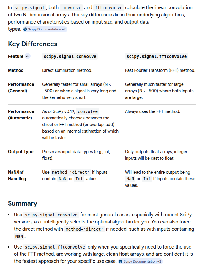
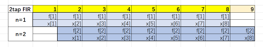
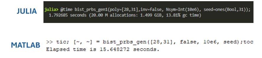
FIR filter typically is much shorter (<10 taps) than the symbol vector, using FFT convolution might be an overkill. For optimization, a simple shift-and-add filter function can be written

function u_filt(So_conv, input, fir; Si_mem=Float64[])
    sconv = zeros(length(input) + length(fir) - 1)

    s_in = lastindex(input)
    
    for n=eachindex(fir)
        sconv[n:s_in+n-1] .+= fir[n] .* input
    end

    sconv[eachindex(Si_mem)] .+= Si_mem

    return sconv
end

PRBS Generator

[https://opencpi.gitlab.io/releases/latest/rst/comp_sdr/components/generator/prbs_generator_b.comp/prbs_generator_b-index.html]

# Julia

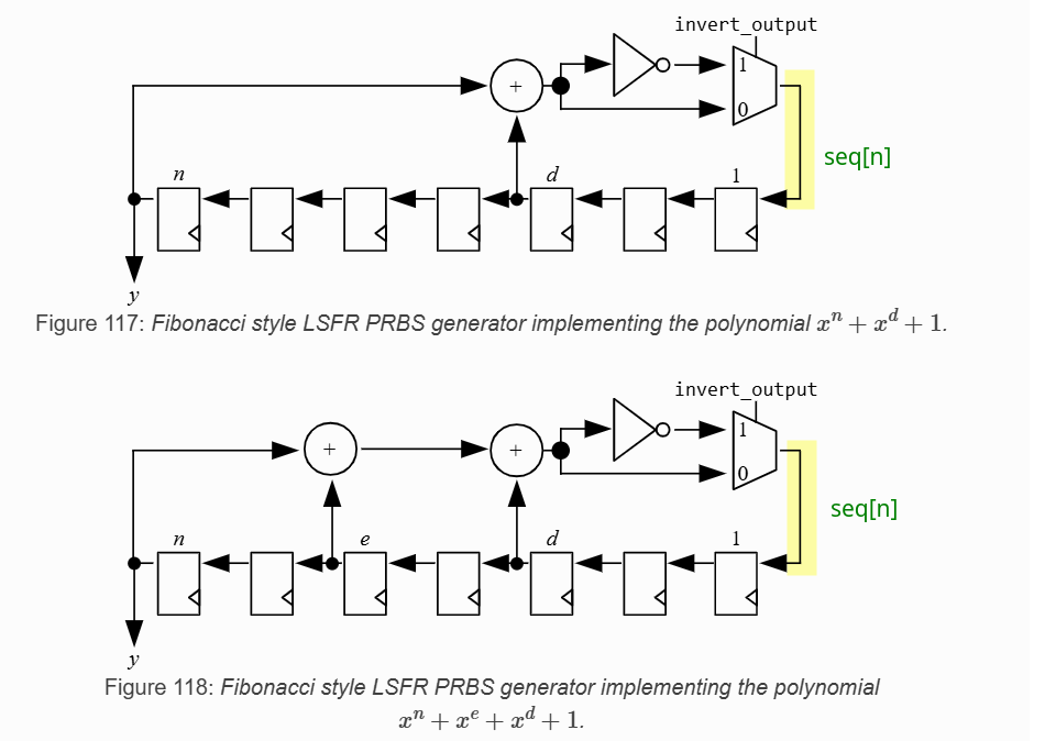
function bist_prbs_gen(;poly, inv, Nsym, seed)
    seq = Vector{Bool}(undef,Nsym)
    for n = 1:Nsym
        seq[n] = inv
        for p in poly
            seq[n] ⊻= seed[p]
        end
        seed .= [seq[n]; seed[1:end-1]]
    end
    return seq, seed
end

%% Matlab

function [seq, seed] = bist_prbs_gen(poly,inv, Nsym, seed)
    seq = zeros(1,Nsym);
    for n = 1:Nsym
        seq(n) = inv;
        for p = poly
            seq(n) = xor(seq(n), seed(p));
        end
       seed = [seq(n), seed(1:end-1)];
    end
end

[https://github.com/kevjzheng/JLSD/blob/main/Pluto%20Notebooks/pdf/JLSD_pt1_background.pdf]

PRBS Checker

[https://github.com/kevjzheng/JLSD/blob/4ac92476b67ce78e01820502eb3b4afb6d31bcd7/Pluto%20Notebooks/jl/JLSD_pt2_framework.jl#L198-L235]

previous bit determine current bit

bert.drawio

current LSFR generate btst
compare bst with current brcv
push current brcv into LSFR

Analog Signals Representation

Ben Yochret Sabrine, 2020, "BEHAVIORAL MODELING WITH SYSTEMVERILOG FOR MIXED-SIGNAL VALIDATION" [https://di.uqo.ca/id/eprint/1224/1/Ben-Yochret_Sabrine_2020_memoire.pdf]

Reference

MATLAB® and Simulink® RF and Mixed Signal [https://www.mathworks.com/help/overview/rf-and-mixed-signal.html]

Lim, Byong Chan, M. Horowitz, "Error Control and Limit Cycle Elimination in Event-Driven Piecewise Linear Analog Functional Models," in IEEE Transactions on Circuits and Systems I: Regular Papers, vol. 63, no. 1, pp. 23-33, Jan. 2016 [https://sci-hub.se/10.1109/TCSI.2015.2512699]

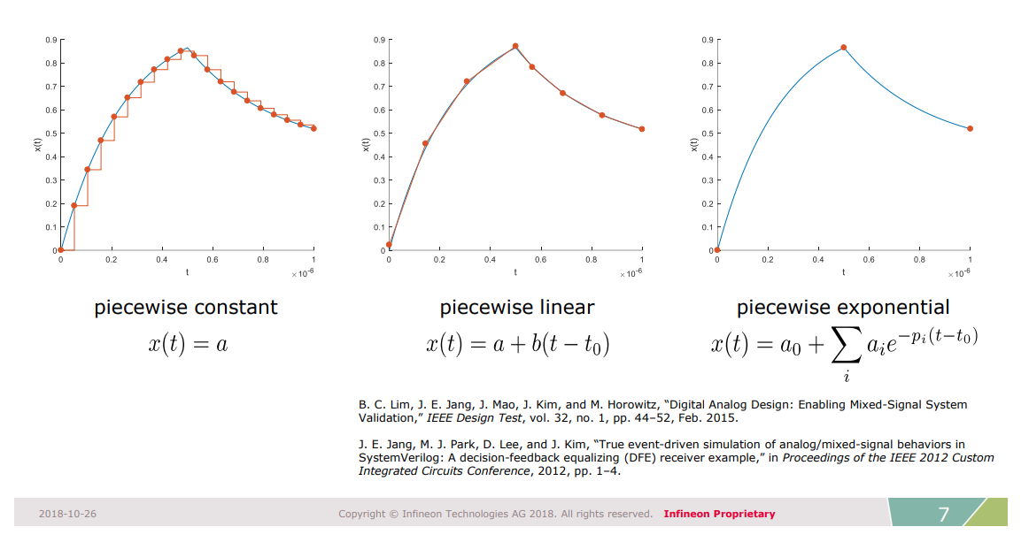
—, Ph.D. Dissertation 2012. "Model validation of mixed-signal systems" [https://stacks.stanford.edu/file/druid:xq068rv3398/bclim-thesis-submission-augmented.pdf]

—, J. -E. Jang, J. Mao, J. Kim and M. Horowitz, "Digital Analog Design: Enabling Mixed-Signal System Validation," in IEEE Design & Test, vol. 32, no. 1, pp. 44-52, Feb. 2015 [http://iot.stanford.edu/pubs/lim-mixed-design15.pdf]

— , Mao, James & Horowitz, Mark & Jang, Ji-Eun & Kim, Jaeha. (2015). Digital Analog Design: Enabling Mixed-Signal System Validation. Design & Test, IEEE. 32. 44-52. [https://iot.stanford.edu/pubs/lim-mixed-design15.pdf]

S. Liao and M. Horowitz, "A Verilog piecewise-linear analog behavior model for mixed-signal validation," Proceedings of the IEEE 2013 Custom Integrated Circuits Conference, San Jose, CA, USA, 2013 [https://sci-hub.se/10.1109/CICC.2013.6658461]

—, M. Horowitz, "A Verilog Piecewise-Linear Analog Behavior Model for Mixed-Signal Validation," in IEEE Transactions on Circuits and Systems I: Regular Papers, vol. 61, no. 8, pp. 2229-2235, Aug. 2014 [https://sci-hub.se/10.1109/TCSI.2014.2332265]

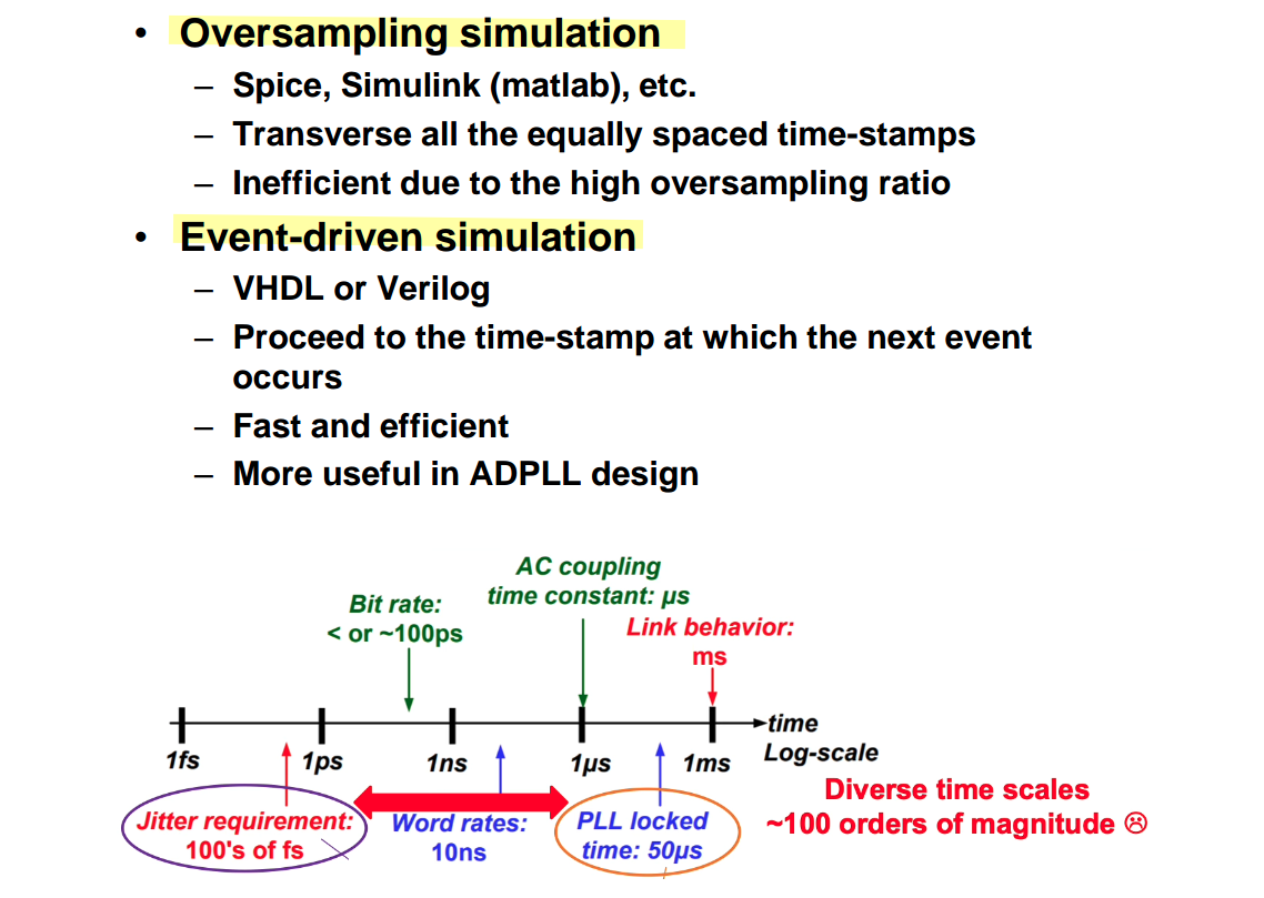
—,Ph.D. Dissertation 2012. Verilog Piecewise Linear Behavioral Modeling For Mixed-Signal Validation [https://stacks.stanford.edu/file/druid:pb381vh2919/Thesis_submission-augmented.pdf]

Ji-Eun Jang et al. “True event-driven simulation of analog/mixed-signal behaviors in SystemVerilog: A decision-feedback equalizing (DFE) receiver example”. In: Proceedings of the IEEE 2012 Custom Integrated Circuits Conference. 2012 [https://sci-hub.se/10.1109/CICC.2012.6330558]

—, Si-Jung Yang, and Jaeha Kim. “Event-driven simulation of Volterra series models in SystemVerilog”. In: Proceedings of the IEEE 2013 Custom Integrated Circuits Conference. 2013 [https://sci-hub.se/10.1109/CICC.2013.6658460]

—, Ph.D. Dissertation 2015. Event-Driven Simulation Methodology for Analog/Mixed-Signal Systems [file:///home/anon/Downloads/000000028723.pdf]

"Creating Analog Behavioral Models VERILOG-AMS ANALOG MODELING" [https://www.eecis.udel.edu/~vsaxena/courses/ece614/Handouts/CDN_Creating_Analog_Behavioral_Models.pdf]

Rainer Findenig, Infineon Technologies. "Behavioral Modeling for SoC Simulation Bridging Analog and Firmware Demands" [https://www.coseda-tech.com/files/Files/Dokumente/Behavioral_Modeling_for_SoC_Simulation_COSEDA_UGM_2018.pdf]

CC Chen. Why Efficient SPICE Simulation Techniques for BB CDR Verification? [https://youtu.be/Z54MV9nuGUI]

T. Wen and T. Kwasniewski, "Phase Noise Simulation and Modeling of ADPLL by SystemVerilog," 2008 IEEE International Behavioral Modeling and Simulation Workshop, San Jose, CA, USA, 2008 [slides, paper]

Jaeha Kim,Scientific Analog. UCIe PHY Modeling and Simulation with XMODEL [pdf]

S. Katare, "Novel Framework for Modelling High Speed Interface Using Python for Architecture Evaluation," 2020 IEEE REGION 10 CONFERENCE (TENCON), Osaka, Japan, 2020 [https://sci-hub.se/10.1109/TENCON50793.2020.9293846]

G. Balamurugan, A. Balankutty and C. -M. Hsu, "56G/112G Link Foundations Standards, Link Budgets & Models," 2019 IEEE Custom Integrated Circuits Conference (CICC), Austin, TX, USA, 2019, pp. 1-95 [https://youtu.be/OABG3u2H2J4] [https://picture.iczhiku.com/resource/ieee/SHKhwYfGotkIymBx.pdf]

Mathuranathan Viswanathan. Digital Modulations using Matlab: Build Simulation Models from Scratch

Time domain modeling

serdespy

JLSD

Sam Palermo's

SerDesSystemCProject

DaVE

Statistical Eye

StatOpt

pystateye

other framework

pyBERT

PyChOpMarg

mmse_dfe

ngscopeclient

SignalIntegrity

Helper Functions

int2bits

generate PAM symbols

eye diagram based on heatmap

FIR by shift-and-add filter

PRBS Generator

PRBS Checker

Analog Signals Representation

Reference

eye diagram based on `heatmap`