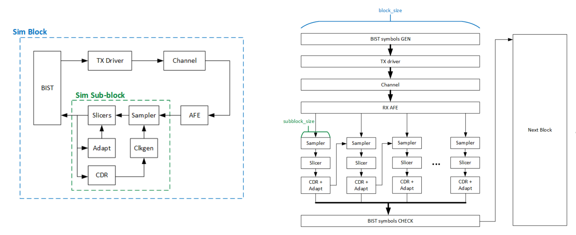
Link Models
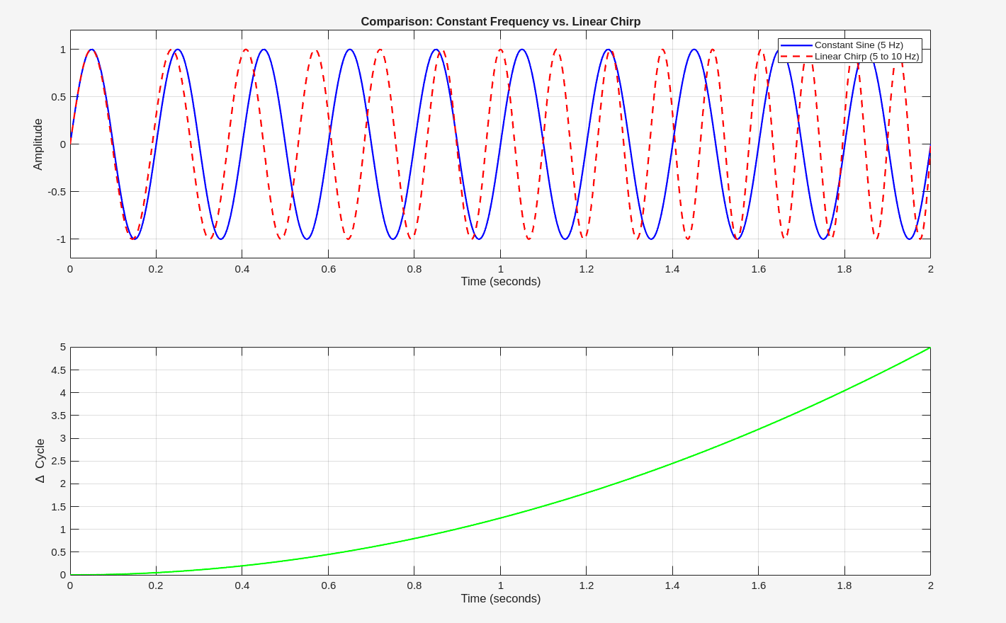
Time domain modeling
While many different analysis methods exist, including frequency and statistical analysis, time domain results remain the final sign-off
serdespy
Richard Barrie. serdespy — A python library for system-level SerDes modelling and simulation [https://github.com/richard259/serdespy]
—, Microelectronics [Introduction to SerDesPy], [Simple Channel Modeling Example with SerDesPy], [Modelling Equalization with SerDesPy]
2
3
pip install samplerate
pip install 'numpy<2.0.0'
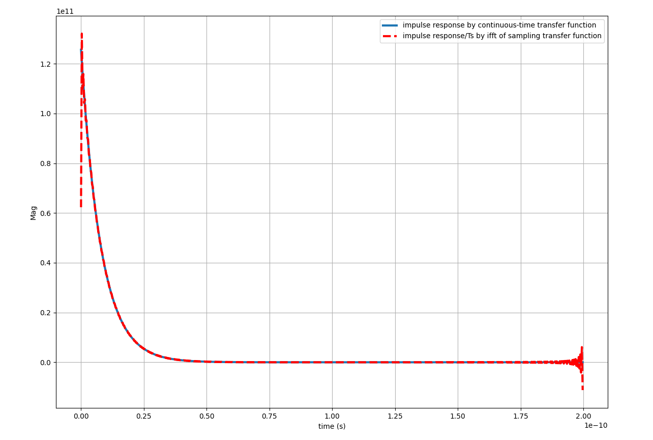
ifft of sampling continuous-time transfer function

1 | def freq2impulse(H, f): |
Maybe, the more straightforward method is sampling impulse response of continuous-time transfer function directly
1 | import numpy as np |
1 | import scipy as sp |
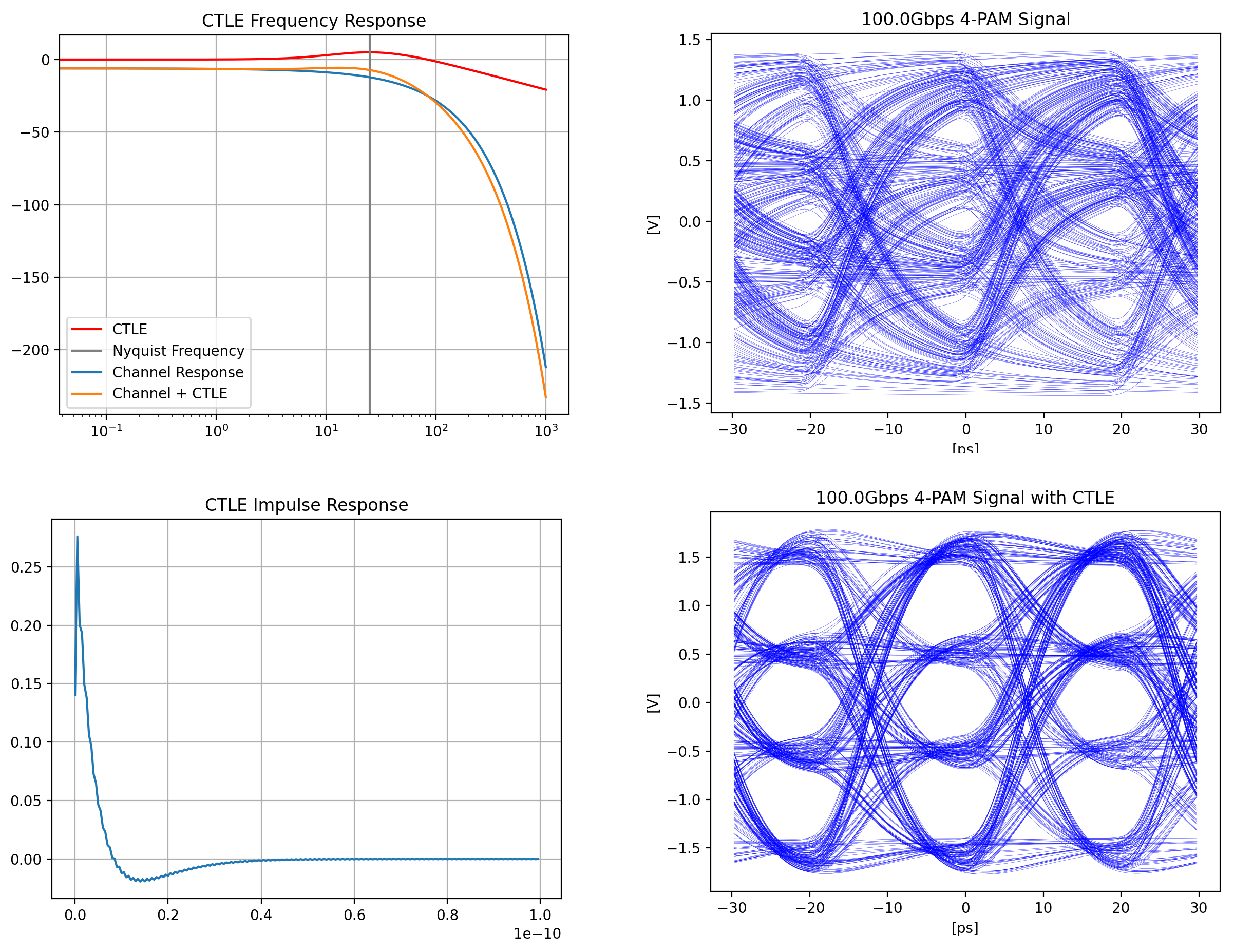
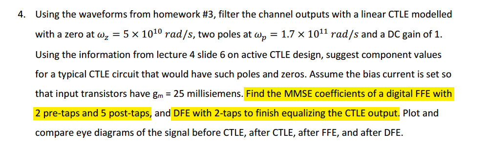
active CTLE
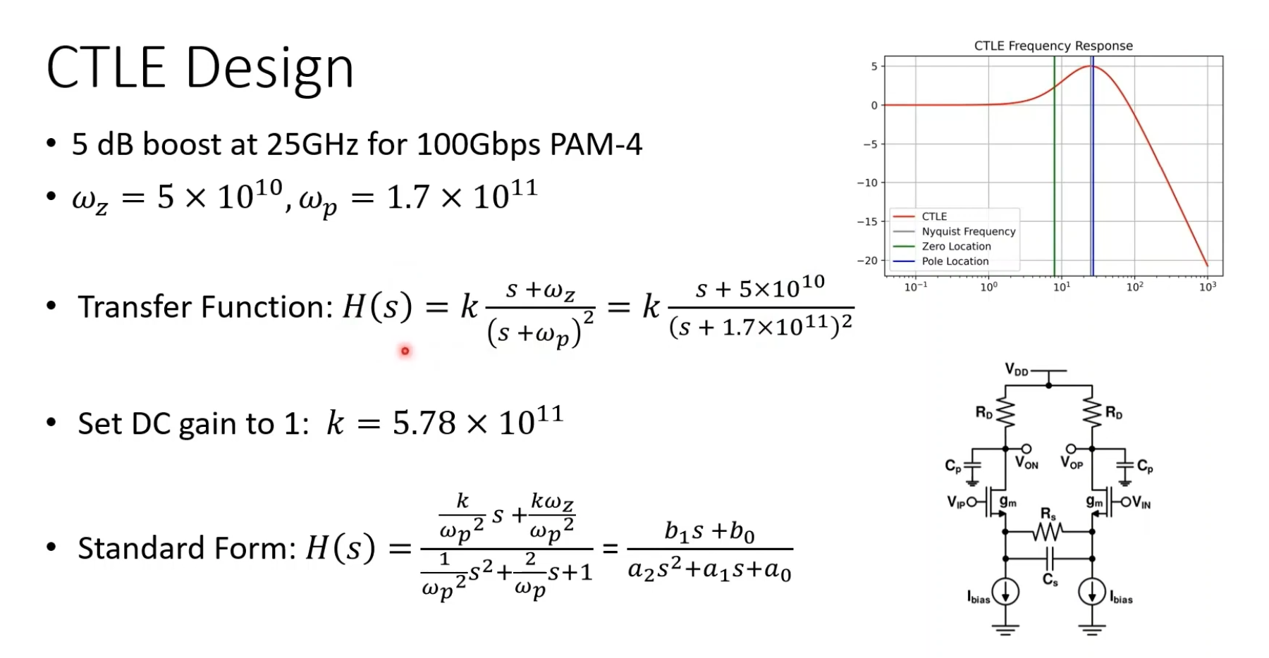
1 | #set poles and zeroes for peaking at nyquist freq |
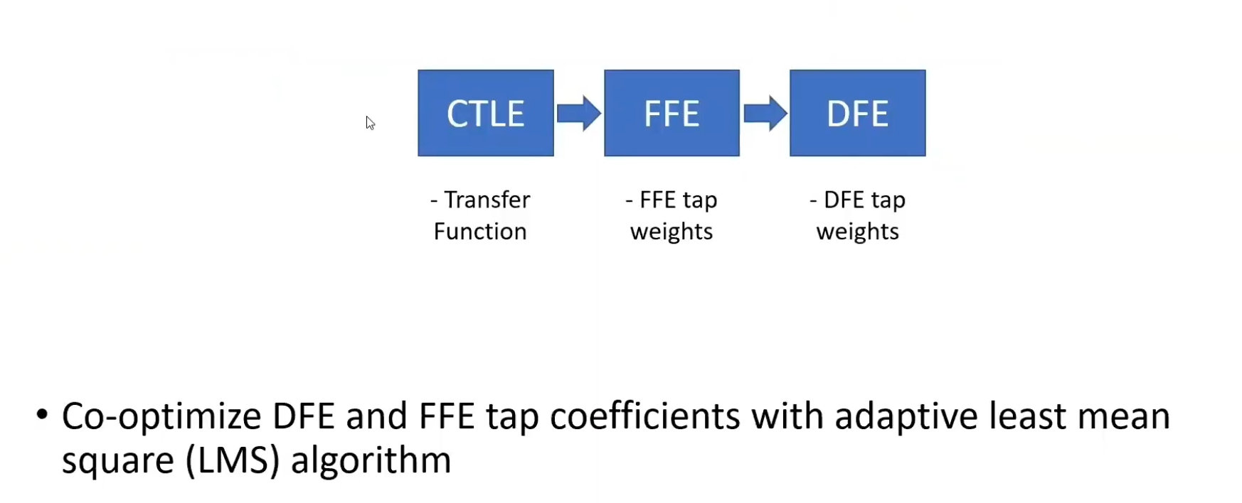
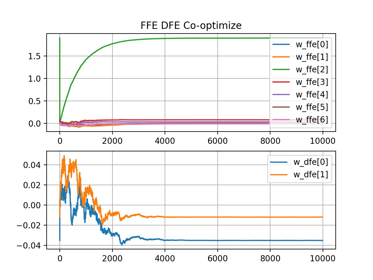
FFE & DFE Co-Optimization with LMS
shift_signal mimic a simple CDR's phase lock
1 | def shift_signal(signal, samples_per_symbol): |
lms_equalizer performs offline
adaptation and it fail due to DFE Error Propagation if
reference is None \[
\underbrace{\mathbf{y}_k}_{\text{FFE input}}
\;\xrightarrow{\;\langle\cdot,\mathbf{w}_{\text{ffe}}\rangle\;}\;
v^{\text{ffe}}_k
\;\xrightarrow{\;-\,\langle\mathbf{z}_k,\mathbf{w}_{\text{dfe}}\rangle\;}\;
v^{\text{dfe}}_k
\;\xrightarrow{\;Q(\cdot)\;}\;
z_k
\]
\[ \boxed{\;\mathbf{w}_{\text{ffe}}^{(k+1)} = \mathbf{w}_{\text{ffe}}^{(k)} - \mu\, e_k\, \mathbf{y}_k\;} \]
\[ \boxed{\mathbf{w}_{\text{dfe}}^{(k+1)} = \mathbf{w}_{\text{dfe}}^{(k)} + \mu\, e_k\, \mathbf{z}_k} \]
1 | def lms_equalizer(y, mu, N, w_ffe, FFE_pre, w_dfe, voltage_levels, |
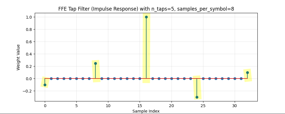
1 | def FFE(self,tap_weights, n_taps_pre): |
1 | # https://github.com/richard259/serdespy/blob/main/serdespy/receiver.py |
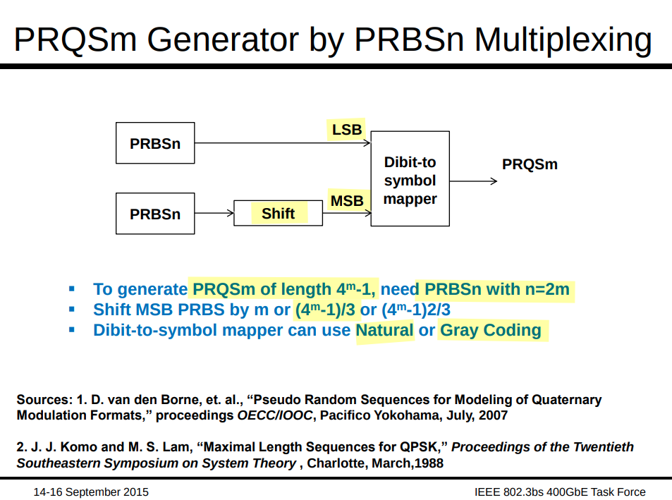
PRQSm Generator by multiplexing two PRBSn
Ilya Lyubomirsky, Finisar. PRQS Test Patterns for PAM4 [https://www.ieee802.org/3/bs/public/15_09/lyubomirsky_3bs_01_0915.pdf]
1 | # https://github.com/richard259/serdespy/blob/main/serdespy/prs.py |
Gaussian distribution jitter
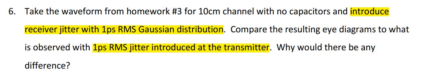
TX signal with jitter

The accuracy of the jitter model is constrained by the
resolution defined as
sample_time = UI/samples_per_symbol within the
gaussian_jitter implementation.
1 | #https://github.com/richard259/serdespy/blob/main/serdespy/transmitter.py |
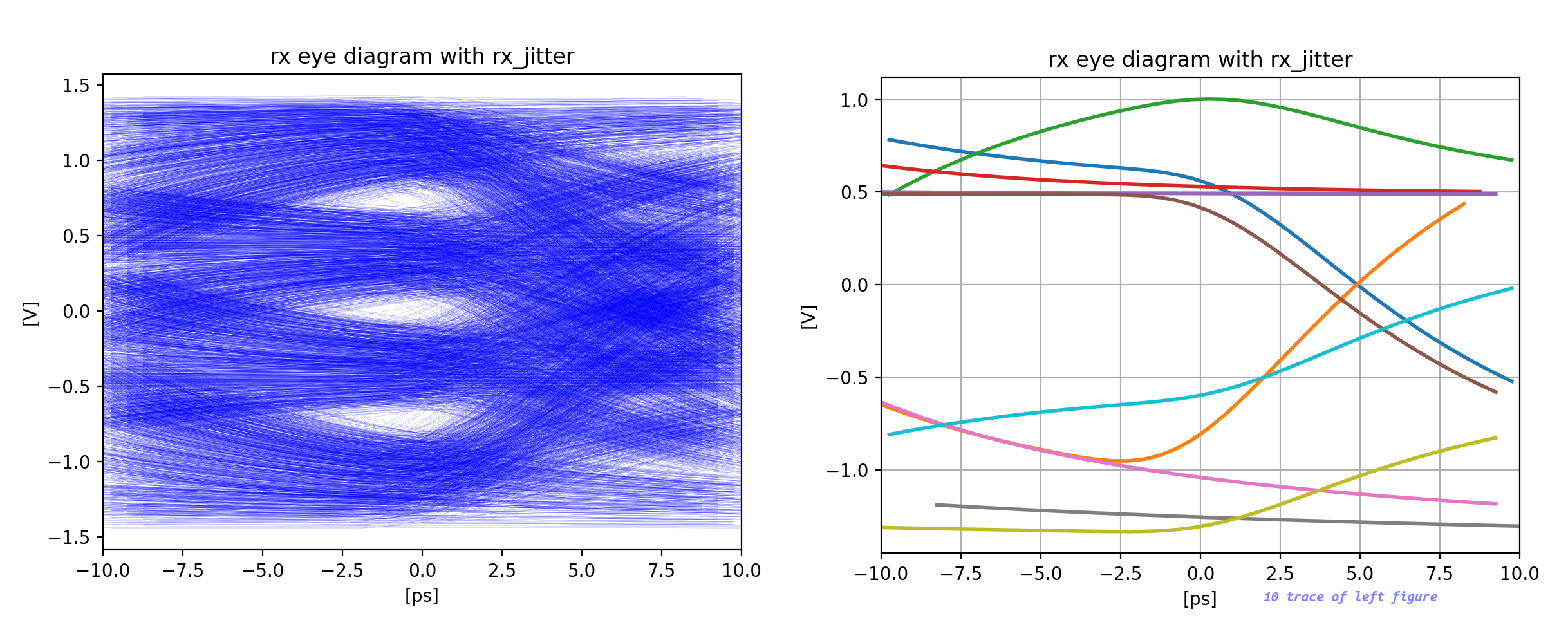
RX eye_diagram with jitter by horizontal shift
Each trace is shifted by its corresponding \(\epsilon\), which is only used for visualization rather than as an input for the subsequent block.
1 | def rx_jitter_eye(signal, window_len, ntraces, n_symbols, tstep, title, stdev, res=600, linewidth=0.15,): |
RLM through nonlinearity
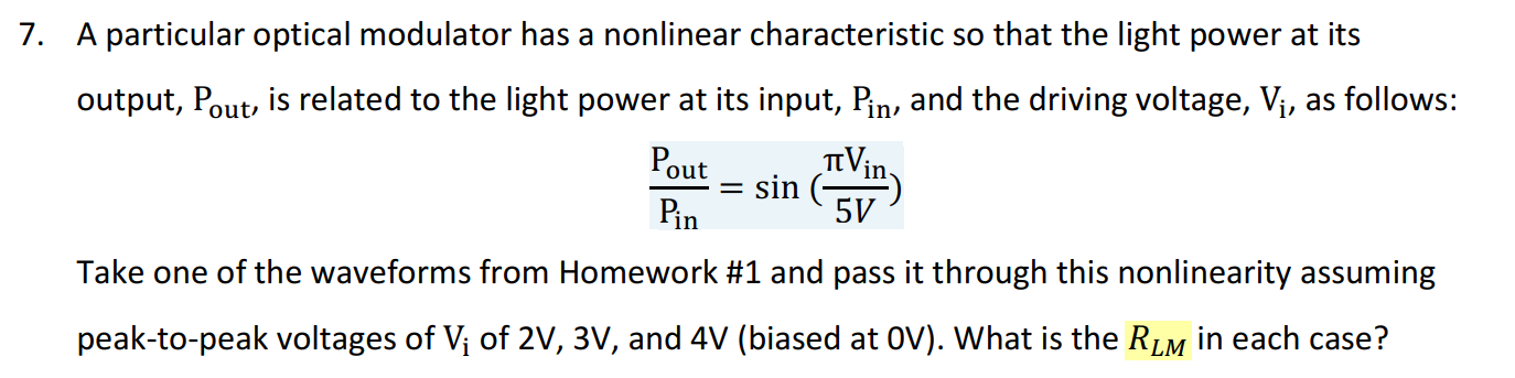
1 | #convolution of impulse response with ideal signal |
JLSD
Kevin Zheng, JLSD - Julia SerDes [https://github.com/kevjzheng/JLSD], [forked]
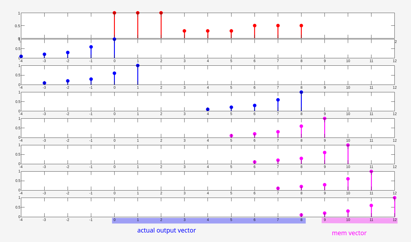
Kronecker product to create oversampled waveform
1 | function gen_wvfm(bits; tui, osr) |

first order RC response, normalized to the time step \[ \frac{\alpha}{s+\alpha} \overset{\mathcal{L}^{-1}}{\longrightarrow} \alpha\cdot e^{-\alpha t} \]
The integral of impulse response of low pass RC filter \(\int_{0}^{+\infty} \alpha\cdot e^{-\alpha t}dt =
1\) — sum(ir*dt)
1 | function gen_ir_rc(dt,bw,t_len) |
sum(ir)*dt = 1, i.e. the step response1
1 | out = conv(ir, vbits)*tui/osr |
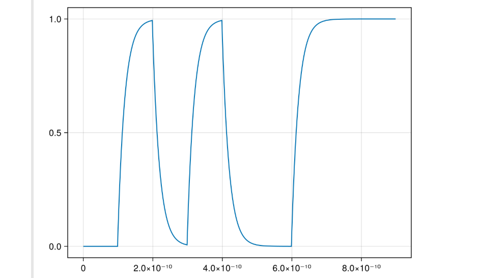
1 | #call our convolution function; let's keep the input memory zero for now |

Detailed Transmitter
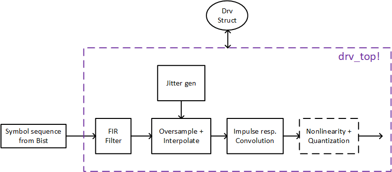
1 | Sfir_conv::Vector = zeros(param.blk_size+length(fir)-1) |
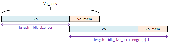
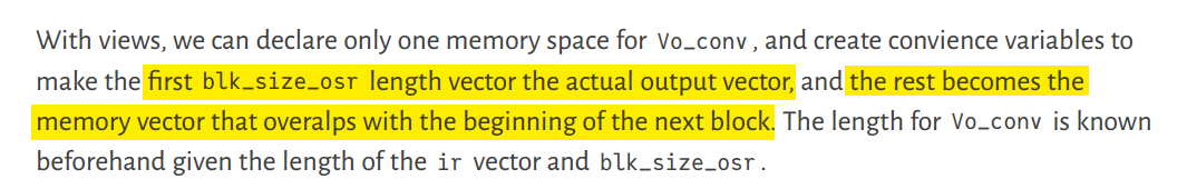
1 | function u_conv!(Vo_conv, input, ir; Vi_mem = Float64[], gain = 1) |
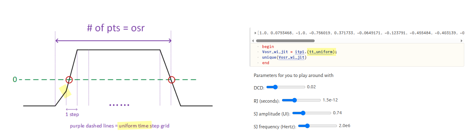
TX model jitter with fixed simulation time step
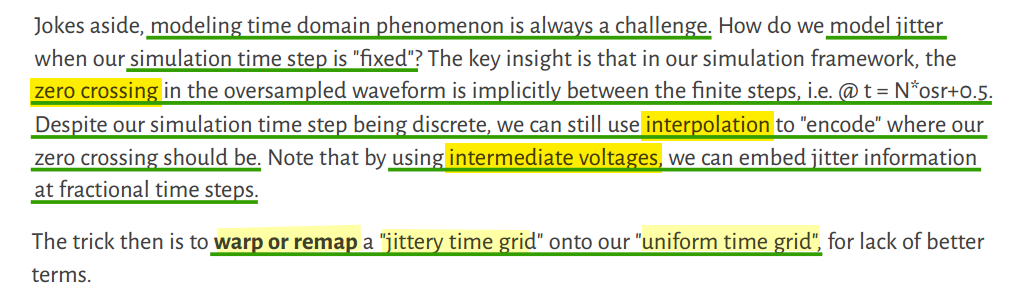
warp or remap a "jittery time grid" onto our "uniform time grid"
The brilliance is that you don't need infinitesimal time steps—instead, you remap the sampling grid to account for jitter!
1 | Vext::Vector = zeros(prev_nui*param.osr+param.blk_size_osr) #(prev_nui + blk_size)*osr |

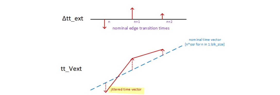
Because each symbol's width is determined by two edges, \(\Delta tt\_\text{ext}\) is is one greater than \(V_\text{ext}\)
1 | function drv_jitter_tvec!(tt_Vext, Δtt_ext, osr) |
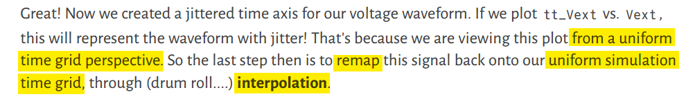
1 | itp = linear_interpolation(drv.tt_Vext, drv.Vext); #itp is a function object |
itp = linear_interpolation(drv.tt_Vext, drv.Vext) create
linear interpolation only, extrapolation shall
not be used to avoid inducing any error
1 | #note here tt_uniform is shifted by prev_nui/2 to give wiggle room for sampling "before" and "after" the current block. This is necessary for sinusoidal jitter |

tt_uniform is shifted by prev_nui/2 to give
wiggle room for sampling "before" and "after" the current block.
This is necessary for sinusoidal jitter
[copilot]
DCD and RJ have much smaller shifts (typically <1 UI), but SJ can oscillate over multiple UI widths, requiring this centered offset to prevent interpolation boundary errors.
1 | function drv_jitter_tvec!(tt_Vext, Δtt_ext, osr) |
This creates tt_Vext starting from
(n-1)*osr, which means:
- First segment:
0*osr + offsetto1*osr + offset= starts at 0 - Second segment:
1*osr + offsetto2*osr + offset - etc.
tt_uniform must align with this same time
scale for interpolation to work correctly.
Starting from 0 ensures tt_uniform
aligns with the OSR sample grid and matches the time values in
tt_Vext for correct interpolation.
1 | function drv_add_jitter!(drv, Vfir) |
In each outer loop, Δtt and Vfir are
created (size blk_size) and then copied into their
respective extended buffers, Δtt_ext and
Vext.


channel
1 | noise_Z::Float64 = 50 # termination impedance with thermal noise |
\[ P_\text{n,dBm/Hz} = 10\times\log_{10} (k_B T / 10^{-3}) = 10\times\log_{10} (k_B T) + 30=-174 \]
Then, \(k_B T = 10^{\frac{-174 - 30}{10}}\)
we have
\[ \sigma_n^2 = 4\cdot k_B T \cdot R \cdot \frac{f_s}{2} = k_B T \cdot R \cdot 2f_s= \frac{\color{red}{2}}{T_s} \cdot 10^{\frac{-174 - 30}{10}} \cdot R \]
noise_rms::Float64 = sqrt(2/param.dt*10^((noise_dbm_hz-30.0)/10)rather thansqrt(0.5/param.dt*10^((noise_dbm_hz-30.0)/10)
Clkgen-PI
1 | mutable struct Clkgen |
| Parameter | Default | Meaning |
|---|---|---|
pi_res |
8 |
PI has 8-bit resolution |
pi_max_code |
2^8 - 1 = 255 |
Code range is 0–255 |
pi_ui_cover |
4 |
The full 256 codes span 4 UI |
pi_codes_per_ui |
2^8 / 4 = 64 |
64 codes per UI |
pi_wrap_ui_Δcode |
255 - 10 = 245 |
Wrap detection threshold |
pi_wrap_ui |
0 |
Starts with zero wraps |
pi_code_prev |
0 |
Previous PI code starts at 0 |
The margin of 10 (pi_max_code - 10)
ensures that even if the CDR makes a moderately large step (up to ±10
codes), it won't be mistaken for a wrap. This is safe as long as the CDR
loop bandwidth is low enough that per-update code changes stay well
below 10
1 | function clkgen_pi_itp_top!(clkgen; pi_code) |
How Wrap Detection Works
1 | PI code: 0 ---------> 255 | 0 ---------> 255 | 0 ---> ... |
| Variable | Role |
|---|---|
pi_wrap_ui |
Accumulated wrap count in UI — keeps Φ0 continuous
across wraps |
Φ0 |
PI-controlled phase offset (CDR tracking loop output) |
pi_wrap_ui accumulates full UI wraps across blocks.
Combined with Φstart = (cur_subblk-1)*subblk_size*osr (the
sub-block offset), this means Φo_subblk coordinates are in
the global sample coordinate system relative to the
start of the current block — which is exactly what
tt_Vext's centered coordinate system expects
1 | function cdr_top!(cdr, Sd, Se) |
Wraps pd_accum into [0, pi_bnd) (i.e.,
[0, 256) for 8-bit PI), then floors it to produce the
integer pi_code that feeds back to
clkgen_pi_itp_top!. This is the modular
accumulator — the same wrapping that
pi_wrap_ui in the clock generator
unwraps.
Sign-Sign Mueller-Muller CDR -
cdr_top!
| pattern | main cursor | Se (assuming \(h_0=\operatorname{dLev}\)) | vote |
|---|---|---|---|
| 011 | \(s_{011}=-h_1+h_0+h_{-1}\) | \(\operatorname{sign}({-h_1+h_{-1}})\) | \(\operatorname{sign}({h_1-h_{-1}})\) |
| 110 | \(s_{110}=h_1+h_0-h_{-1}\) | \(\operatorname{sign}({h_1-h_{-1}})\) | \(\operatorname{sign}({h_1-h_{-1}})\) |

sampler
1 | mutable struct Splr |
This is where the two approaches are inverted:
| Drv (TX jitter) | Splr (RX sampling) | |
|---|---|---|
tt_Vext |
Non-uniform (jittered) | Uniform (fixed) |
Vext values |
Uniform voltage samples | Uniform voltage samples |
| Query points | tt_uniform — fixed grid |
Φi from CDR — variable clock
phases |
| Interpolation | Jittered-time → uniform-time | Uniform-time → CDR-phase |
| Direction | Resample onto sim grid | Sample at recovered clock instants |
tt_uniform is offset by prev_nui/2 * osr to
land in the center of Vext, giving
prev_nui/2 = 2 UIs of headroom on each side for jitter
excursions.
1 | Φ = osr*(pi_wrap_ui + pi_code/pi_codes_per_ui) + Φnom + Φskew + Φrj |
These Φ values are in the same coordinate system as
tt_Vext. Because tt_Vext is centered
(-8*osr ... 8*osr + blk_size_osr - 1), the nominal sampling
phases at 0, osr, 2*osr, ... fall right in the center of
the buffer
Different prev_nui Sizes
| Drv | Splr | |
|---|---|---|
prev_nui |
4 | 16 |
| Headroom per side | 2 UIs | 8 UIs |
| Reason | TX jitter is bounded (DCD ≪ 1UI, RJ/SJ typically < 1UI) | CDR PI can accumulate large phase offsets over time
(pi_wrap_ui multiples of 4 UI) |
adaptation and CDR loop
1 | ## pseudo-code |
clkgen = TrxStruct.Clkgen(nphases = 4, skews = [0e-12, 0e-12, 0e-12, 0e-12])dslc = TrxStruct.Slicers(N_per_phi = ones(UInt8, clkgen.nphases), dac_min = -0.1, dac_max = 0.1)eslc = TrxStruct.Slicers(N_per_phi = UInt8.([1,0,0,0]),dac_min = 0, dac_max = 0.5)cdr = TrxStruct.Cdr(Neslc_per_phi = eslc.N_per_phi)adpt = TrxStruct.Adpt(Neslc_per_phi = eslc.N_per_phi
1 | mutable struct Splr |
\(\operatorname{dLev}\) adaptation \[ dLev_{n+1} = dLev_n + \mu\cdot \operatorname{sign}( e_n) \]
1 | function adpt_top!(adpt, Sd, Se) |
dslc.So & eslc.So
initialization with Number of comparisons
executed during each phase N_per_phi
1 | mutable struct Slicers |
For DSLC: N_per_phi=[1,1,1,1]
1 | dslc.So = [zeros(Bool, Int(N_per_phi[n%nphases+1])) for n in 0:param.subblk_size-1] |
For ESLC: N_per_phi=[1,0,0,0]
1 | eslc.So = [zeros(Bool, Int(N_per_phi[n%nphases+1])) for n in 0:param.subblk_size-1] |
elastic buffer to model frequency offsets of TRX
elastic buffer — an analog waveform window for the RX
sampler, not a digital FIFO
Define the offset relative to TX \[f_\text{rx} = f_\text{tx}(1 + \text{ppm}\cdot 10^{-6})\], RX sample spacing in TX-grid units \[ \boxed{\text{osr}_\text{rx} = \dfrac{\text{osr}}{1+\text{ppm}\cdot 10^{-6}}} \]
The inner loop's exit condition (ignoring \(\phi0\)/jitter for a moment) is: \[ n_\text{available} < (\text{subblk}_\text{size} - 1)\cdot\text{osr}_\text{rx} + 1 \approx \text{subblk}_\text{size}\cdot\text{osr}_\text{rx} \] So at every exit point of the inner loop, buffer occupancy is strictly less than one sub-block's worth.
\[ \Phi_0^{\text{legacy}} = \text{osr}\cdot\bigl(\text{pi\_wrap\_ui} + \text{pi\_code}/\text{pi\_codes\_per\_ui}\bigr) \]
1 | % 1. Define Parameters |
Sam Palermo's
continuous time filter (channel, ctle); impulse response
digital filter (FFE, DFE): repmat by samples per UI
Sam Palermo. ECEN 720: High-Speed Links Circuits and Systems [https://people.engr.tamu.edu/spalermo/ecen720.html]
repmat
1 | >> repmat([1,2,3], 3, 1) |
1 | >> reshape(repmat([1,2,3], 3, 1), 1, 3*3) |
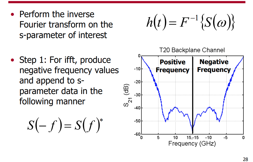
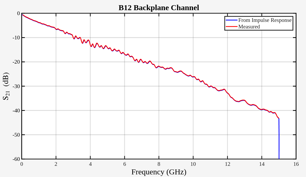
Generating an Impulse Response from S-Parameters
ECEN720: High-Speed Links Circuits and Systems Spring 2025 [https://people.engr.tamu.edu/spalermo/ecen689/lecture3_ee720_tdr_spar.pdf]
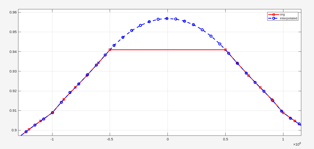
spline: Cubic spline data interpolation
2
3
4
5
6
figure(Name='spline function')
plot(fds_m, Hm_ds, '-rs', LineWidth=2)
hold on
plot(f_ds_interp, Hm_ds_interp, '--bo', LineWidth=2)
legend('org', 'interpolated'); grid on
impulse response from ifft of interpolated frequency response
1 | % https://people.engr.tamu.edu/spalermo/ecen689/xfr_fn_to_imp.m |
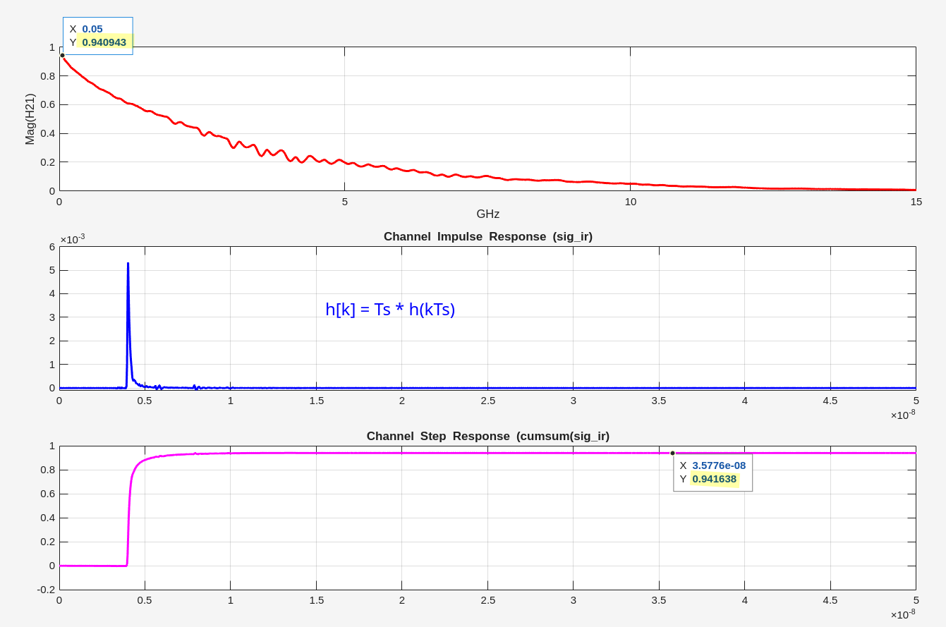
1 | subplot(3,1,1) |
2
legend('From Impulse Response','Measured');
plot eye diagram
1 | % https://people.engr.tamu.edu/spalermo/ecen689/channel_data.m |
If your 2D array represents multiple data series (e.g., each column is a separate line series sharing the same x-axis values), the
plot()function is the most straightforward method.
[https://people.engr.tamu.edu/spalermo/ecen689/lecture4_ee720_channel_pulse_model.pdf]
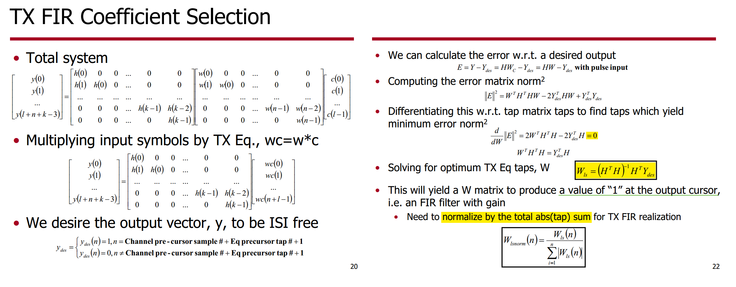
1 | % https://people.engr.tamu.edu/spalermo/ecen689/tx_eq.m |
TX FIR Tap Resolution
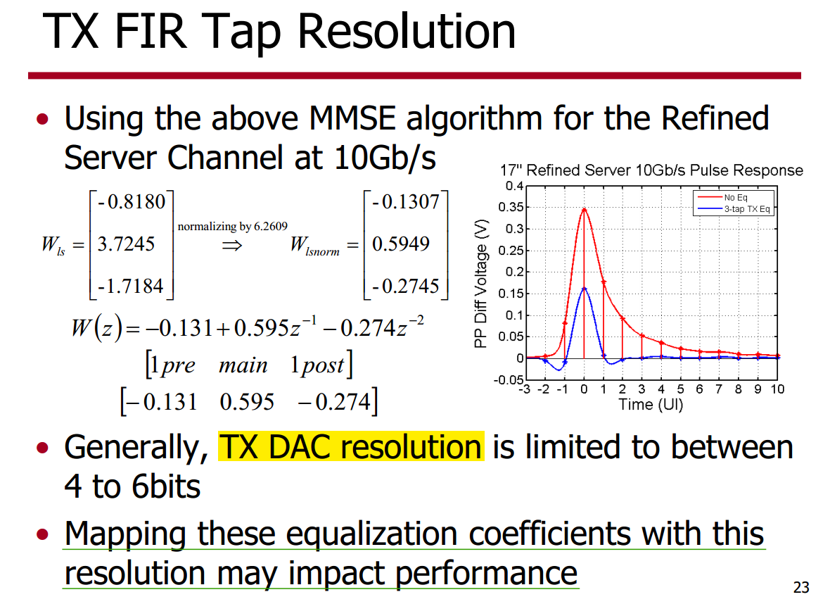
1 | % https://people.engr.tamu.edu/spalermo/ecen689/tx_eq.m |
CTLE modeling by impulse response
Given two impulse response \(h_0(t)\), \(h_1(t)\) and \(h_0(t)*h_1(t) = h_{tot}(t)\), we have \[ T_s h_0(kT_s) * T_sh_1(kT_s) = T_s h_{tot}(kT_s) \]
To use the
filterfunction with thebcoefficients from an FIR filter, usey = filter(b,1,x)
CTLE response from frequency response using
ifft
data-driven frequency table
1 | % https://people.engr.tamu.edu/spalermo/ecen689/gen_ctle.m |
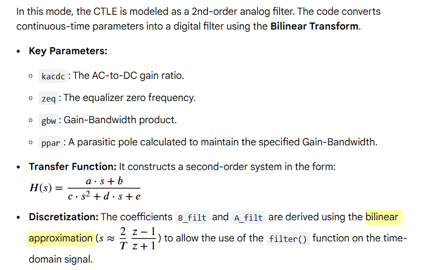
CTLE response from pole/zero using
tf & impulse
1 | H21 = tf(); |
CTLE response from pole/zero using
bilinear discretization
analytical pole/zero transfer function, [Google AI Mode]

1 | % https://people.engr.tamu.edu/spalermo/ecen689/gen_ctle.m |
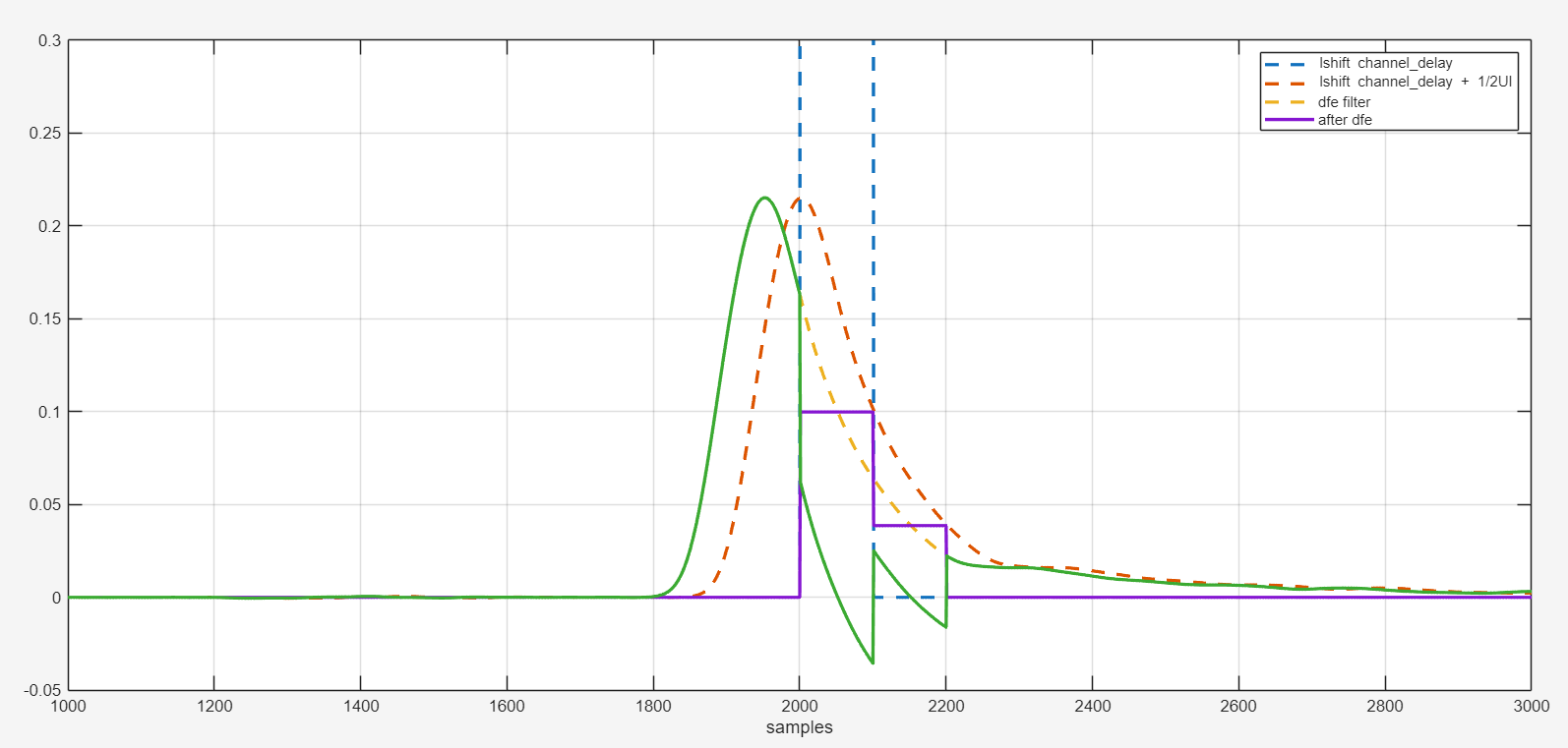
rx dfe
pseudo linear equalizer
1 | % https://people.engr.tamu.edu/spalermo/ecen689/channel_data_pulse_pda_dfe.m |
2
3
4
5
6
7
plot(data_channel(channel_delay:end), '--', LineWidth=2)
hold on
plot(data_channel(channel_delay+dfe_fb_offset:channel_delay+dfe_fb_offset+size(m_dfe_dr,2)-1), '--', LineWidth=2)
plot(m_dfe_dr, LineWidth=2); plot(data_channel_dfe, LineWidth=2)
xlim([1000, 3000]); ylim([-0.05, 0.3]); xlabel('samples'); grid on
legend('lshift channel\_delay', 'lshift channel\_delay + 1/2UI', 'dfe filter', 'after dfe')
SerDesSystemCProject
Lewis Liu [https://github.com/LewisLiuLiuLiu/SerDesSystemCProject]
sasasatori, SystemC简介与安装 [https://www.cnblogs.com/sasasatori/p/17865550.html]
Rahul Bhadani. [SystemC-AMS Quick Installation Guide] [SystemC Quick Installation Guide]
SerDes - High-Speed Serial Link Simulator (SystemC-AMS)
1 | """ |
Install SystemC
1 | ## CMakeLists.txt |
test systemc
1 | cmake_minimum_required(VERSION 3.0) |
Install SystemC-AMS
1 | mkdir build && cd build |
DaVE
Byongchan Lim. DaVE — tools regarding on analog modeling, validation, and generation, [https://github.com/StanfordVLSI/DaVE]
TODO 📅
Statistical Eye
Sanders, Anthony, Michael Resso and John D'Ambrosia. “Channel Compliance Testing Utilizing Novel Statistical Eye Methodology.” (2004) [https://people.engr.tamu.edu/spalermo/ecen689/stateye_theory_sanders_designcon_2004.pdf]
X. Chu, W. Guo, J. Wang, F. Wu, Y. Luo and Y. Li, "Fast and Accurate Estimation of Statistical Eye Diagram for Nonlinear High-Speed Links," in IEEE Transactions on Very Large Scale Integration (VLSI) Systems, vol. 29, no. 7, pp. 1370-1378, July 2021 [https://sci-hub.se/10.1109/TVLSI.2021.3082208]
IA Title: Common Electrical I/O (CEI) - Electrical and Jitter Interoperability agreements for 6G+ bps, 11G+ bps, 25G+ bps I/O and 56G+ bps IA # OIF-CEI-04.0 December 29, 2017 [pdf]
J. Park and D. Kim, "Statistical Eye Diagrams for High-Speed Interconnects of Packages: A Review," in IEEE Access, vol. 12, pp. 22880-22891, 2024 [pdf]
StatOpt
Jeremy Cosson-Martin, Jhoan Salinas, Savo Bajic, and Ali Sheikholeslami, January 2024, StatOpt: A Statistical Eye Analysis and Link Optimization Tool [https://www.eecg.utoronto.ca/~ali/statopt/main.html]
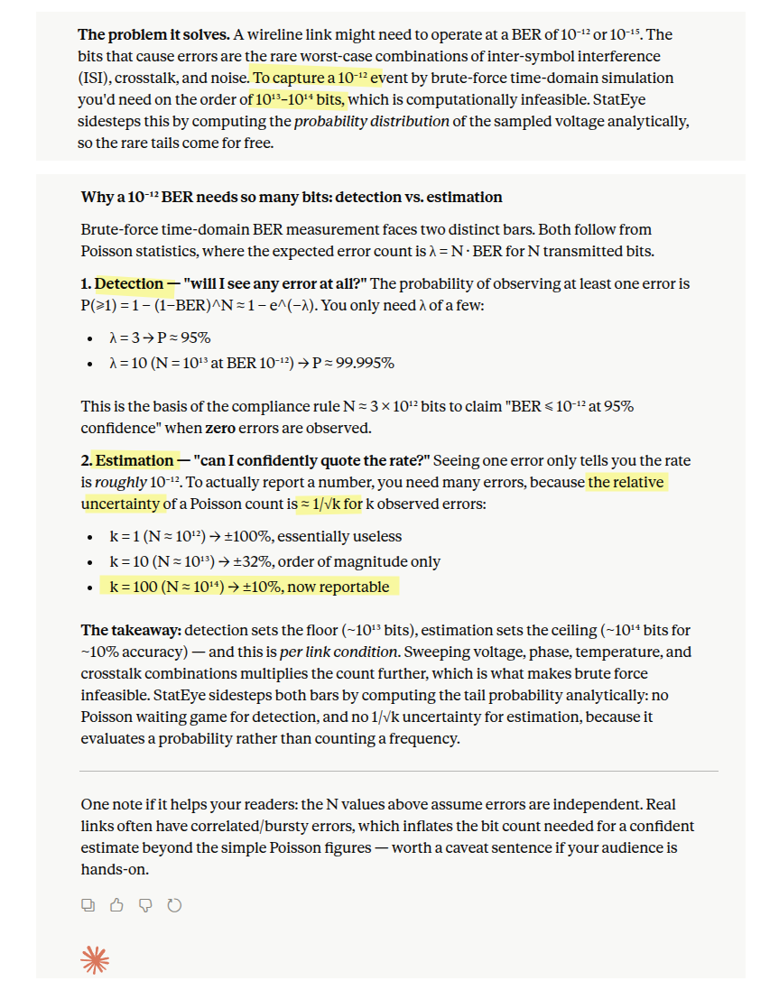
StatOpt is a statistical eye analysis and link optimization tool for wireline communications, developed in both MATLAB and Python 3
The tool uses statistical methods to model various wireline effects and to estimate the link performance metrics such as the bit error rate and eye dimensions (eye's horizontal and vertical openings)

High-Level Pipeline
flowchart TD
    A["User Settings<br/>(GenerateUserSettingsExampleN)"] --> B["Settings Limits<br/>(GenerateSettingsLimits)"]
    B --> C["Initialize Simulation<br/>(InitializeSimulation)"]
    C --> D["Check Settings<br/>(CheckSettings)"]
    D --> E["Fixed Influences<br/>(GenerateFixedInfluence)"]
    E --> F{"Adaptation Loop<br/>while ~finished"}

    F --> G["Variable Influences<br/>(GenerateVariableInfluence)"]
    G --> H["Pulse Response<br/>(GeneratePulseResponse)"]
    H --> I["ISI Trajectories<br/>(GenerateISI)"]
    I --> J["PDF Eye Diagram<br/>(GeneratePDF)"]
    J --> K["BER Contours<br/>(GenerateBER)"]
    K --> L["Results / Measurements<br/>(GenerateResults)"]
    L --> M["Adapt Link<br/>(AdaptLink)"]
    M -->|not finished| F
    M -->|finished| N["Display Plots<br/>(Display* functions)"]
Every function reads from and writes to two MATLAB structs that flow through the entire pipeline:
| Struct | Purpose |
|---|---|
simSettings |
All user-configurable knobs + derived constants. Populated once at startup; mutated only by the adaptation engine. |
simResults |
Accumulates all computed data: channel responses, jitter/noise PDFs, pulse responses, ISI trajectories, PDF/BER eye diagrams, measurements, and adaptation state. |
Fixed Influences (runs once) —
GenerateFixedInfluence.m
Computes channel and impairment data that does not change across adaptation iterations:
flowchart LR
    A["CreateChannel"] --> B["GenerateTXJitter"]
    B --> C["GenerateTXDistortion"]
    C --> D["GenerateRXJitter"]
    D --> E["GenerateRXDistortion"]
    E --> F["CombineInfluences"]
Variable Influences —
GenerateVariableInfluence.m
omputes impairment sources that depend on equalization settings (and thus change during adaptation):
| Sub-function | What it computes |
|---|---|
| GenerateCTLE | CTLE transfer function from zero/pole specs (cached to avoid recomputation) |
| CalculateFFERMS | RMS of FFE tap values (needed for noise output-referring) |
| GenerateTXNoise | TX noise → attenuated through channel → amplified by CTLE/FFE → Gaussian PDF at RX output |
| GenerateChannelNoise | Thermal noise → amplified by CTLE/FFE → Gaussian PDF |
| GenerateRXNoise | RX input-referred noise → amplified by pre-amp/CTLE/FFE → Gaussian PDF |
| CombineInfluences | Convolves TX + channel + RX noise PDFs into total noise PDF |
Noise is output-referred — each noise source is propagated through the downstream signal chain (channel, CTLE, FFE) before creating the probability distribution. This is why noise must be recomputed when equalization changes.
Pulse Response —
GeneratePulseResponse.m
Builds the end-to-end pulse response through the full signal chain:
flowchart LR
A["ApplyPulse<br/>(ideal pulse)"] --> B["ApplyTXEQ<br/>(FIR pre-emphasis)"]
B --> C["ApplyChannel<br/>(convolution with channel IR)"]
C --> D["ApplyRXGain<br/>(pre-amplifier)"]
D --> E["ApplyRXCTLE<br/>(continuous-time EQ via lsim)"]
E --> F["ApplyRXFFE<br/>(FIR equalization)"]
F --> G["ApplyRXDFE<br/>(post-cursor subtraction)"]
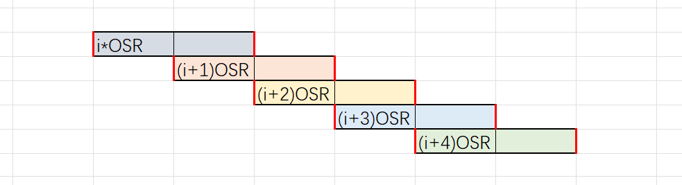
G --> H["LimitLength<br/>(trim to cursor window)"]ISI Generation —
GenerateISI.m
Generates all possible signal trajectories due to inter-symbol interference:
- GenerateCursorCombinations — Enumerates all
M^Ncursor patterns (M = modulation levels, N = cursor count) - ClassifyTrajectories — Groups combinations by their
main-cursor transition type (e.g.,
trans01,trans10) - SplitPulse — Slices the pulse response into per-cursor segments
- ApplyCursorCombination — For each combination, multiplies cursors by data levels and sums → one trajectory per combination
Computational complexity is O(M^N) — for PAM-4 with 7
cursors this is 4^7=16384 combinations. Reducing cursor
count speeds up simulation at the cost of accuracy
PDF Generation —
GeneratePDF.m
Builds the statistical eye diagram by layering impairments onto the ISI distribution:
flowchart LR
    A["GenerateHist<br/>(ISI → voltage histograms)"] --> B["ApplyCrossTalk<br/>(vertical convolution)"]
    B --> C["ApplyDistortion<br/>(voltage remapping)"]
    C --> D["ApplyJitter<br/>(horizontal convolution)"]
    D --> E["ApplyNoise<br/>(vertical convolution)"]
    E --> F["CombinePDFs<br/>(merge all transitions)"]
Each step creates a new named PDF layer (e.g.,
PDF.initial, PDF.crossTalk,
PDF.distorted, PDF.jitter,
PDF.noise, PDF.final), enabling intermediate
visualization.
Adaptation — AdaptLink.m
If simSettings.adaption.adapt = false, sets
finished = true and the loop exits after one pass.
If enabled, implements a genetic algorithm with three modes:
flowchart LR
    A["Mode 1: Coarse Search<br/>(±3 increments, N generations)"] --> B["Mode 2: Fine Search<br/>(±1 increment, N generations)"]
    B --> C["Mode 3: Final Run<br/>(restore full settings, run optimal)"]
Python Version of StatOpt
Savo Bajic, ECE1392, Integrated Circuits for Digital Communications: StatOpt in Python [https://savobajic.ca/projects/academic/statopt]
[https://github.com/savob/statopt-python]
https://www.eecg.utoronto.ca/~ali/statopt/StatOptPython.html]
pyBERT
David Banas. pyBERT: Free software for signal-integrity analysis [https://github.com/capn-freako/PyBERT], [intro]
—. Free yourself from IBIS-AMI models with PyBERT [https://www.edn.com/free-yourself-from-ibis-ami-models-with-pybert/]
TODO 📅
CTLE model
flowchart TD
    Start([get_ctle_h]) --> UseFile{self.use_ctle_file?}

    UseFile -->|Yes: load from file| Import["ctle_h = import_channel(ctle_file, ts, f)"]
    Import --> StepChk{"max(abs(ctle_h)) < 100.0?<br/>(step response?)"}
    StepChk -->|Yes| Diff["ctle_h = diff(ctle_h)<br/>impulse = d/dt of step"]
    StepChk -->|No| Norm["ctle_h *= ts<br/>normalize to V/sample"]
    Diff --> Pad["ctle_h = resize_zero_pad(ctle_h, len_t)"]
    Norm --> Pad
    Pad --> Fft["ctle_H = rfft(ctle_h)<br/>(freq-domain; ToDo: needs interp)"]
    Fft --> Ret([return ctle_h])

    UseFile -->|No: native model| EnaChk{ctle_enable?}

    EnaChk -->|Yes| Make["_, ctle_H = make_ctle(rx_bw, peak_freq, peak_mag, w)<br/>build freq response from EQ params"]
    Make --> Irfft["_ctle_h = irfft(ctle_H)<br/>back to time domain"]
    Irfft --> Interp["krnl = interp1d(t_irfft, _ctle_h, fill=0)<br/>ctle_h = krnl(t)<br/>resample onto sim time grid t"]
    Interp --> Gain["ctle_h *= sum(_ctle_h)/sum(ctle_h)<br/>preserve DC gain after resample"]
    Gain --> Trim["ctle_h, _ = trim_impulse(ctle_h, ...)<br/>crop negligible tail"]
    Trim --> Ret

    EnaChk -->|No: bypass| Ident["ctle_h = [1., 0., 0., ...]<br/>unit impulse (pass-through)"]
    Ident --> Ret

    style StepChk fill:#ffb74d,stroke:#e65100,stroke-width:2px,color:#000
    style Diff fill:#a5d6a7,stroke:#2e7d32,stroke-width:2px,color:#000
    style Norm fill:#a5d6a7,stroke:#2e7d32,stroke-width:2px,color:#000
    style Gain fill:#ffb74d,stroke:#e65100,stroke-width:2px,color:#000
ctle_h *= sum(_ctle_h) / sum(ctle_h) : preserve
DC gain after resample
1 | def get_ctle_h(): |
pystateye
Chris Li. pystateye - A Python Implementation of Statistical Eye Analysis and Visualization [https://github.com/ChrisZonghaoLi/pystateye]
TODO 📅
SeaSim
Seasim (Statistical Eye Analysis Simulator) is a statistical channel simulation tool provided by the PCI-SIG to help designers evaluate the signal integrity and compliance of PCI Express (PCIe) links
other tools
IBIS-AMI
Init mode — Statistical (Fast) :
1 | Channel |
GetWave mode Time-domain (Slow but more realistic):
1 | Bit stream |
PyChOpMarg
David Banas. Python implementation of COM, as per IEEE 802.3-22 Annex 93A. [https://github.com/capn-freako/PyChOpMarg]
—, COM: A Link Designer's Field Guide [https://www.signalintegrityjournal.com/articles/3578-com-a-link-designers-field-guide]
CC Chen. Why Channel Operating Margin? [https://youtu.be/mrXur-WbrR8]
Python implementation of IEEE Ethernet COM (Channel Operating Margin)
TODO 📅
mmse_dfe
Chris Li, jointly optimizing feed-forward equalizer (FFE) and decision-feedback equalizer (DFE) tap weights [https://github.com/ChrisZonghaoLi/mmse_dfe]
John M. Cioffi, Chapter 3 - Equalization [https://cioffi-group.stanford.edu/doc/book/chap3.pdf]
TODO 📅
ngscopeclient
TODO 📅
SignalIntegrity
SignalIntegrity: Signal and Power Integrity Tools [https://github.com/Nubis-Communications/SignalIntegrity]
TODO 📅
helper functions
int2bits
1 | function int2bits(num, nbit) |
generate PAM symbols
here Big Endian
1 | #generate PAM symbols |
1 | function int2bits(num, nbit) |
eye diagram based on
heatmap
1 | function w_gen_eye_simple_test(input,x_npts_ui, x_npts, y_range, y_npts; osr, x_ofst=0) |
Julia's interpolation return a function object that can operate on any values you throw at it

1 | function u_hist(samples, minval, maxval, nbin) |
FIR by shift-and-add filter
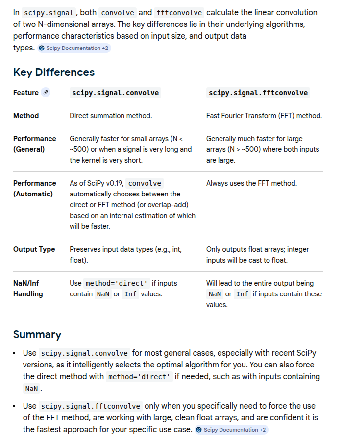
FIR filter typically is much shorter (<10 taps) than the symbol vector, using FFT convolution might be an overkill. For optimization, a simple shift-and-add filter function can be written
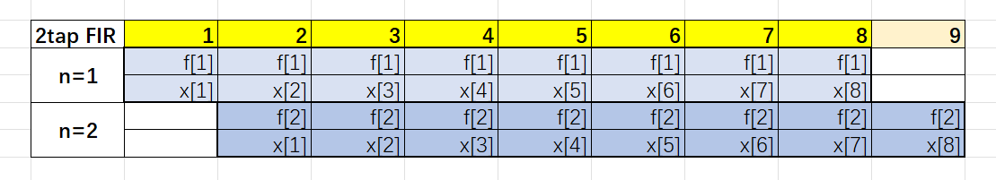
1 | function u_filt(So_conv, input, fir; Si_mem=Float64[]) |
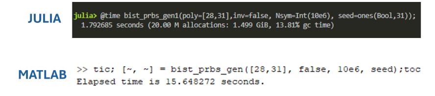
PRBS Generator
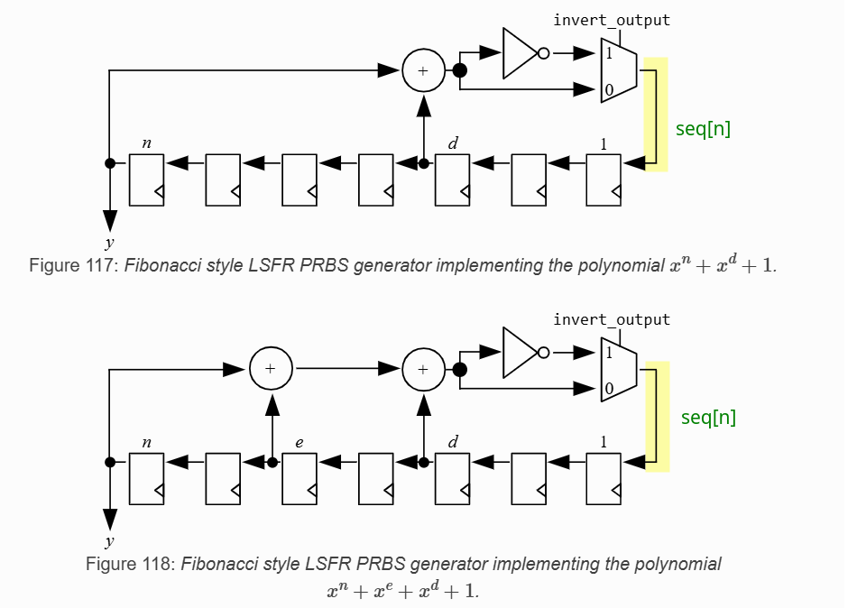
1 | # Julia |
1 | %% Matlab |
[https://github.com/kevjzheng/JLSD/blob/main/Pluto%20Notebooks/pdf/JLSD_pt1_background.pdf]
PRBS Checker
previous bit determine current bit

- current LSFR generate
btst - compare
bstwith currentbrcv - push current
brcvinto LSFR
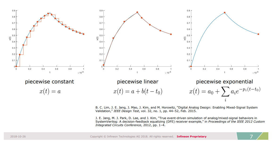
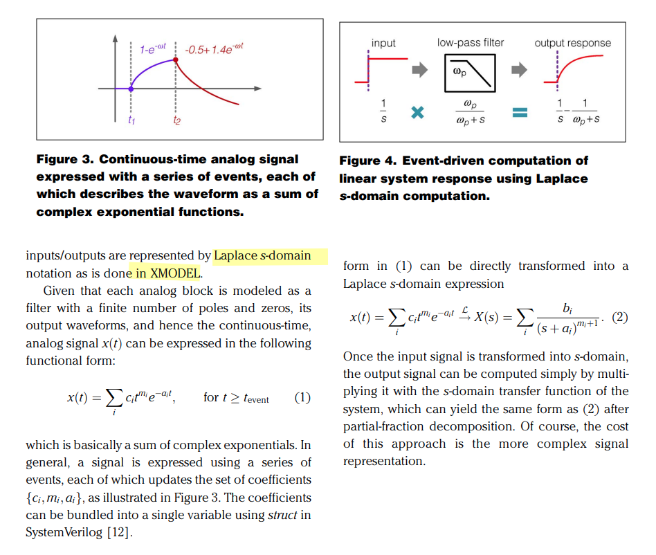
Analog Signals Representation
Ben Yochret Sabrine, 2020, "BEHAVIORAL MODELING WITH SYSTEMVERILOG FOR MIXED-SIGNAL VALIDATION" [https://di.uqo.ca/id/eprint/1224/1/Ben-Yochret_Sabrine_2020_memoire.pdf]
Reference
MATLAB® and Simulink® RF and Mixed Signal [https://www.mathworks.com/help/overview/rf-and-mixed-signal.html]
Lim, Byong Chan, M. Horowitz, "Error Control and Limit Cycle Elimination in Event-Driven Piecewise Linear Analog Functional Models," in IEEE Transactions on Circuits and Systems I: Regular Papers, vol. 63, no. 1, pp. 23-33, Jan. 2016 [https://sci-hub.se/10.1109/TCSI.2015.2512699]
—, Ph.D. Dissertation 2012. "Model validation of mixed-signal systems" [https://stacks.stanford.edu/file/druid:xq068rv3398/bclim-thesis-submission-augmented.pdf]
—, J. -E. Jang, J. Mao, J. Kim and M. Horowitz, "Digital Analog Design: Enabling Mixed-Signal System Validation," in IEEE Design & Test, vol. 32, no. 1, pp. 44-52, Feb. 2015 [http://iot.stanford.edu/pubs/lim-mixed-design15.pdf]
— , Mao, James & Horowitz, Mark & Jang, Ji-Eun & Kim, Jaeha. (2015). Digital Analog Design: Enabling Mixed-Signal System Validation. Design & Test, IEEE. 32. 44-52. [https://iot.stanford.edu/pubs/lim-mixed-design15.pdf]
S. Liao and M. Horowitz, "A Verilog piecewise-linear analog behavior model for mixed-signal validation," Proceedings of the IEEE 2013 Custom Integrated Circuits Conference, San Jose, CA, USA, 2013 [https://sci-hub.se/10.1109/CICC.2013.6658461]
—, M. Horowitz, "A Verilog Piecewise-Linear Analog Behavior Model for Mixed-Signal Validation," in IEEE Transactions on Circuits and Systems I: Regular Papers, vol. 61, no. 8, pp. 2229-2235, Aug. 2014 [https://sci-hub.se/10.1109/TCSI.2014.2332265]
—,Ph.D. Dissertation 2012. Verilog Piecewise Linear Behavioral Modeling For Mixed-Signal Validation [https://stacks.stanford.edu/file/druid:pb381vh2919/Thesis_submission-augmented.pdf]
Ji-Eun Jang et al. “True event-driven simulation of analog/mixed-signal behaviors in SystemVerilog: A decision-feedback equalizing (DFE) receiver example”. In: Proceedings of the IEEE 2012 Custom Integrated Circuits Conference. 2012 [https://sci-hub.se/10.1109/CICC.2012.6330558]
—, Si-Jung Yang, and Jaeha Kim. “Event-driven simulation of Volterra series models in SystemVerilog”. In: Proceedings of the IEEE 2013 Custom Integrated Circuits Conference. 2013 [https://sci-hub.se/10.1109/CICC.2013.6658460]
—, Ph.D. Dissertation 2015. Event-Driven Simulation Methodology for Analog/Mixed-Signal Systems [file:///home/anon/Downloads/000000028723.pdf]
"Creating Analog Behavioral Models VERILOG-AMS ANALOG MODELING" [https://www.eecis.udel.edu/~vsaxena/courses/ece614/Handouts/CDN_Creating_Analog_Behavioral_Models.pdf]
Rainer Findenig, Infineon Technologies. "Behavioral Modeling for SoC Simulation Bridging Analog and Firmware Demands" [https://www.coseda-tech.com/files/Files/Dokumente/Behavioral_Modeling_for_SoC_Simulation_COSEDA_UGM_2018.pdf]
CC Chen. Why Efficient SPICE Simulation Techniques for BB CDR Verification? [https://youtu.be/Z54MV9nuGUI]
T. Wen and T. Kwasniewski, "Phase Noise Simulation and Modeling of ADPLL by SystemVerilog," 2008 IEEE International Behavioral Modeling and Simulation Workshop, San Jose, CA, USA, 2008 [slides, paper]
Jaeha Kim,Scientific Analog. UCIe PHY Modeling and Simulation with XMODEL [pdf]
S. Katare, "Novel Framework for Modelling High Speed Interface Using Python for Architecture Evaluation," 2020 IEEE REGION 10 CONFERENCE (TENCON), Osaka, Japan, 2020 [https://sci-hub.se/10.1109/TENCON50793.2020.9293846]
G. Balamurugan, A. Balankutty and C. -M. Hsu, "56G/112G Link Foundations Standards, Link Budgets & Models," 2019 IEEE Custom Integrated Circuits Conference (CICC), Austin, TX, USA, 2019, pp. 1-95 [https://youtu.be/OABG3u2H2J4] [https://picture.iczhiku.com/resource/ieee/SHKhwYfGotkIymBx.pdf]
Mathuranathan Viswanathan. Digital Modulations using Matlab: Build Simulation Models from Scratch