Zero(DC component) and Nyquist Component in FFT

DC offset

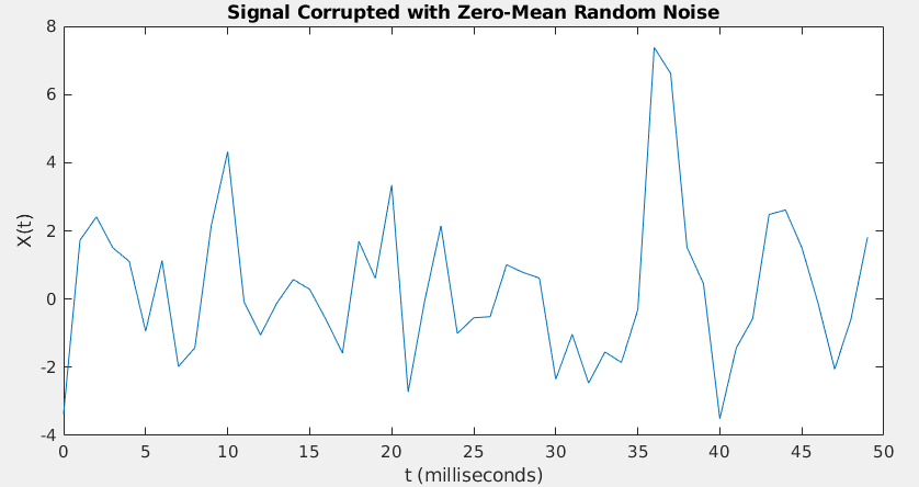
Performing FFT to a signal with a large DC offset would often result in a big impulse around frequency 0 Hz, thus masking out the signals of interests with relatively small amplitude.

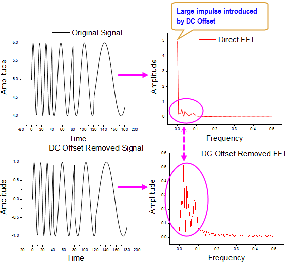
One method to remove DC offset from the original signal before performing FFT

• Subtracting the Mean of Original Signal

You can also not filter the input, but set zero to the zero frequency point for FFT result.

Nyquist component

If we go back to the definition of the DFT \[ X(N/2)=\sum_{n=0}^{N-1}x[n]e^{-j2\pi (N/2)n/2}=\sum_{n=0}^{N-1}x[n]e^{-j\pi n}=\sum_{n=0}^{N-1}x[n](-1)^n \] which is a real number.

The discrete function \[ x[n]=\cos(\pi n) \] is always \((-1)^n\) for integer \(n\)

One general sinusoid at Nyquist and has phase shift \(\theta\), this is \(T=2\) and \(T_s=1\)

\[\begin{align} x[n] &= A \cos(\pi n + \theta) \\ &= A \big( \cos(\pi n) \cos(\theta) - \sin(\pi n) \sin(\theta) \big) \\ &= \big(A\cos(\theta)\big) \cos(\pi n) + \big(-A\sin(\theta)\big) \sin(\pi n) \\ &= \big(A\cos(\theta)\big) (-1)^n + \big(-A\sin(\theta)\big) \cdot 0 \\ &= B \cdot (-1)^n \\ \end{align}\]

Where \(A\cos(\theta)=B\).

Moreover \(B \cdot (-1)^n = B\cdot \cos(\pi n)\), then \[ B\cdot \cos(\pi n) = A \cdot \cos(\pi n + \theta) \] We can NOT distinguish one from another.

In other words, you CAN'T infer the signal from \(X(\frac{N}{2})\) \[\begin{align} X(k)\frac{1}{N}e^{j 2 \pi \frac{nk}{N}}\bigg|_{k=\frac{N}{2}} &= \frac{X\left(\frac{N}{2} \right)}{N}(-1)^n \\ &= \frac{X\left(\frac{N}{2} \right)}{N}\cos(\pi n) \\ &= \frac{X\left(\frac{N}{2} \right)}{N}\left( \cos(\pi n) - \beta \sin(\pi n) \right) \\ &= \frac{X\left(\frac{N}{2} \right)}{N}\sqrt{1+\beta^2}\left(\frac{1}{\sqrt{1+\beta^2}} \cos(\pi n) - \frac{\beta}{\sqrt{1+\beta^2}} \sin(\pi n) \right) \\ &= \frac{X\left(\frac{N}{2} \right)}{N} \frac{1}{\cos(\theta)}\left(\cos(\theta) \cos(\pi n) - \sin(\theta) \sin(\pi n) \right) \\ &= \frac{X\left(\frac{N}{2} \right)}{N} \frac{1}{\cos(\theta)} \cos(\pi n+\theta) \end{align}\]

where \(\beta \in \mathbb{R}\) and you wouldn't know it because \(\sin(\pi n)=0 \quad \forall n \in \mathbb{Z}\)

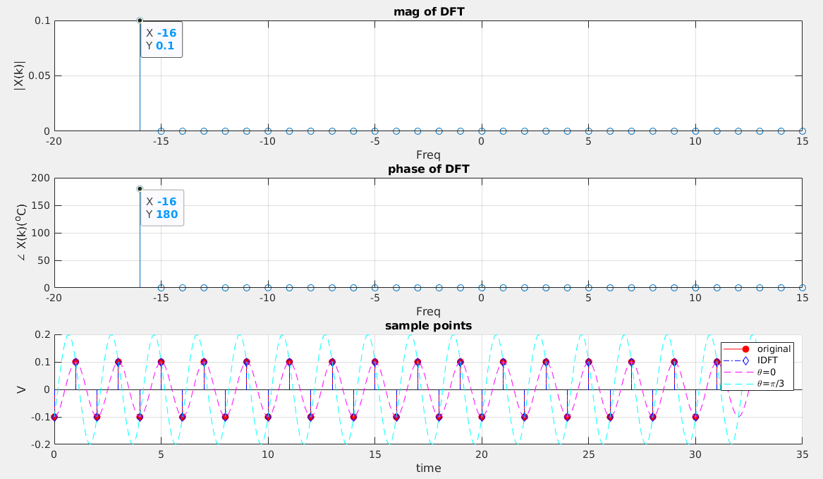
For example, if \(\theta=0\) \[ X(k)\frac{1}{N}e^{j 2 \pi \frac{nk}{N}}\bigg|_{k=\frac{N}{2}}= \frac{X\left(\frac{N}{2} \right)}{N} \cos(\pi n) \] However, if \(\theta=\frac{\pi}{3}\) \[ X(k)\frac{1}{N}e^{j 2 \pi \frac{nk}{N}}\bigg|_{k=\frac{N}{2}}= \frac{X\left(\frac{N}{2} \right)}{N}\cdot 2 \cos(\pi n+\frac{\pi}{3}) \]

That sort of ambiguity is the reason for the strict inequality of the sampling theorem's condition.

Duty Cycle Distortion

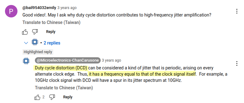
Both edges is used for clock waveform to evaluate the duty cycle distortion,

Assuming TIE is [0 0.2 0 0.2 0 0.2 ...], then subtract DC offset, we get [-0.1 0.1 -0.1 0.1 ...], shown as below

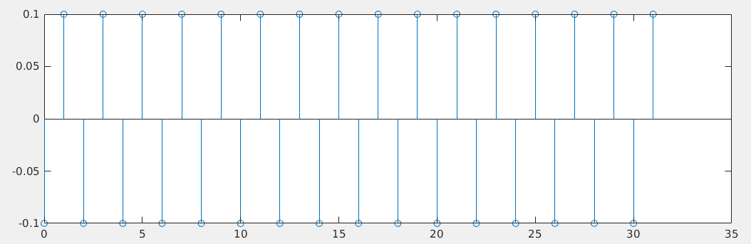
The amplitude is manifested in FFT amplitude spectrum, i.e. Nyquist component, which is 0.1 in follow figure

N = 32;
n = (1:N);
x = 0.1*(-1).^n;
figure(1)
stem(n-1, x);
X = fft(x)/N;
Xshift = fftshift(X);
fprintf("nyquist component: %.2f\n", Xshift(1));
magXshift = abs(Xshift);
ph = phase(Xshift)/pi*180;
figure(2)
subplot(3, 1, 1)
fx = (-N/2:N/2-1);
stem(fx, magXshift);
xlabel('Freq');
ylabel('|X(k)|');
title('mag of DFT');
grid on;

subplot(3, 1, 2)
stem(fx, ph);
xlabel('Freq');
ylabel('\angle X(k)(^oC)');
title('phase of DFT');
grid on;

%% inverse dft
ninv = (0:32-1);
xinv = Xshift(1)*cos(pi*ninv);
subplot(3, 1, 3);
hold on;
stem(ninv, x, "filled", 'r');
stem(ninv, xinv,'bd-.');
ninfer = (0:0.1:32+1);
xinfer1 = Xshift(1)*cos(pi*ninfer); % theta = 0
xinfer2 = Xshift(1)*2*cos(pi*ninfer+pi/3); % theta = pi/3
plot(ninfer, xinfer1, 'm--');
plot(ninfer, xinfer2, 'c--');
hold off;
legend('original', 'IDFT', '\theta=0', '\theta=\pi/3');
xlabel('time');
ylabel('V');
title('sample points');
grid on;

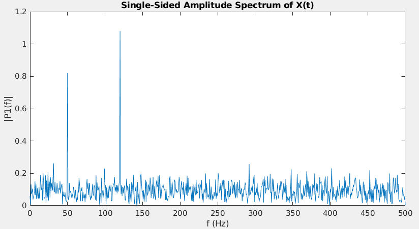
Single-Sided Amplitude Spectrum

DC and Nyquist frequency of FFT left over

P1(2:end-1) = 2*P1(2:end-1);

Fs = 1000;            % Sampling frequency
T = 1/Fs;             % Sampling period
L = 1500;             % Length of signal
t = (0:L-1)*T;        % Time vector
S = 0.7*sin(2*pi*50*t) + sin(2*pi*120*t);
X = S + 2*randn(size(t));
figure(1)
plot(1000*t(1:50),X(1:50))
title('Signal Corrupted with Zero-Mean Random Noise')
xlabel('t (milliseconds)')
ylabel('X(t)')

figure(2)
Y = fft(X);
P2 = abs(Y/L);      %!!! two-sided spectrum P2.
P1 = P2(1:L/2+1);   %!!! single-sided spectrum P1
P1(2:end-1) = 2*P1(2:end-1);	% exclude DC and Nyquist freqency
f = Fs*(0:(L/2))/L;
figure(2)
plot(f,P1)
title('Single-Sided Amplitude Spectrum of X(t)')
xlabel('f (Hz)')
ylabel('|P1(f)|')

Alternative View

The direct current (DC) bin (\(k=0\)) and the bin at \(k=N/2\), i.e., the bin that corresponds to the Nyquist frequency are purely real and unique.

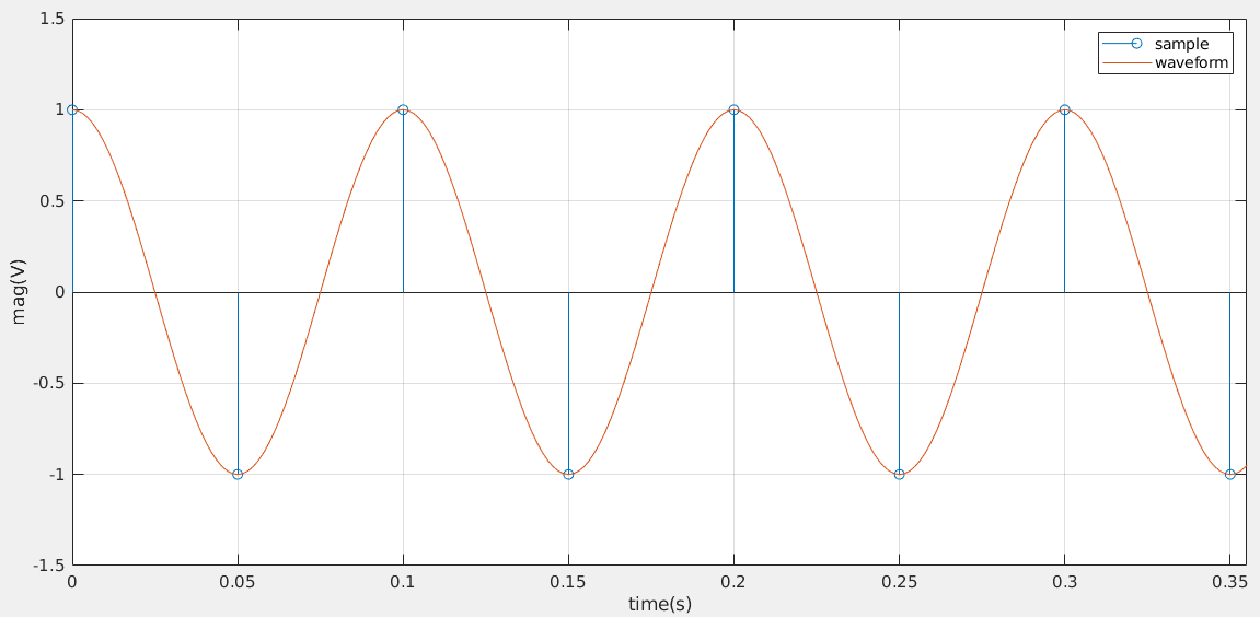
sinusoidal waveform with \(10Hz\), amplitude 1 is \(cos(2\pi f_c t)\). The plot is shown as below with sampling frequency is \(20Hz\)

Amplitude and Phase spectrum, sampled with \(f_s=20\) Hz

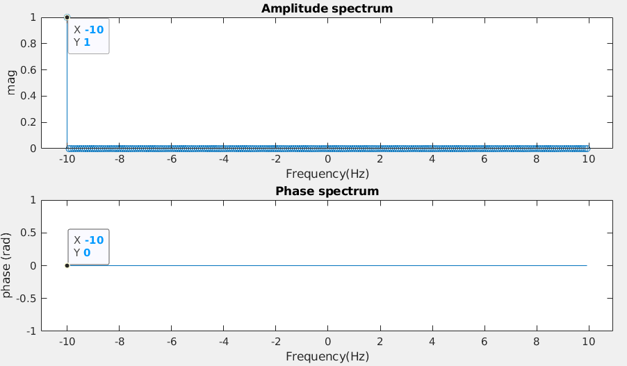
The FFT magnitude of \(10Hz\) is 1 and its phase is 0 as shown as above, which proves the DFT and IDFT.

Caution: the power of FFT is related to samples (DFT Parseval's theorem), which may not be the power of continuous signal. The average power of samples is ([1 -1 1 -1 -1 1 ...]) is 1, that of corresponding continuous signal is \(\frac{1}{2}\).

Power spectrum derived from FFT provide information of samples, i.e. 1

Moreover, average power of sample [1 -1 1 -1 1 ...] is same with DC [1 1 1 1 ...].

code

fc = 10;
fs = 2*fc;
fov = 64*fc;

ts = (0:1/fs:26);
tov = (0:1/fov:26);

ys = cos(2*pi*fc*ts);
yov = cos(2*pi*fc*tov);
%% waveform
stem(ts, ys)
hold on;
plot(tov, yov);
legend('sample', 'waveform')
ylim([-1.5 1.5])
grid on;
xlabel('time(s)');
ylabel('mag(V)')

nfft = 256;
X = fftshift(fft(ys, nfft))/nfft;
f = (-nfft/2:nfft/2-1)*fs/nfft;
magX = abs(X);
phsX = atan2(imag(X),real(X));
%% fft spectrum
figure(2)
subplot(2, 1, 1);
stem(f, magX);
xlabel('Frequency(Hz)');
ylabel('mag')
xlim([min(f)-1 max(f)+1])
title('Amplitude spectrum')
subplot(2, 1, 2)
plot(f, phsX);
xlabel('Frequency(Hz)');
ylabel('phase (rad)')
xlim([min(f)-1 max(f)+1])
title('Phase spectrum')

%% power spectrum
yssq_sum_avg = sum(ys(1:nfft).^2)/nfft;
specsq_sum_avg = sum(abs(X).^2);

reference

OriginLab, How to Remove DC Offset before Performing FFT URL: http://blog.originlab.com/how-to-remove-dc-offset-before-performing-fft

How to remove DC component in FFT? URL: https://www.mathworks.com/matlabcentral/answers/712808-how-to-remove-dc-component-in-fft#answer_594373

Analyzing a signal that contains frequency content at Fs/2 doesn't seem to work unless there is a phase shift URL: https://dsp.stackexchange.com/a/59807/59253

Nyquist–Shannon sampling theorem, Critical frequency URL: https://en.wikipedia.org/wiki/Nyquist%E2%80%93Shannon_sampling_theorem#Critical_frequency

Why remove energy at Nyquist before ifft? URL: https://dsp.stackexchange.com/a/22851/59253