Jitter Decomposition
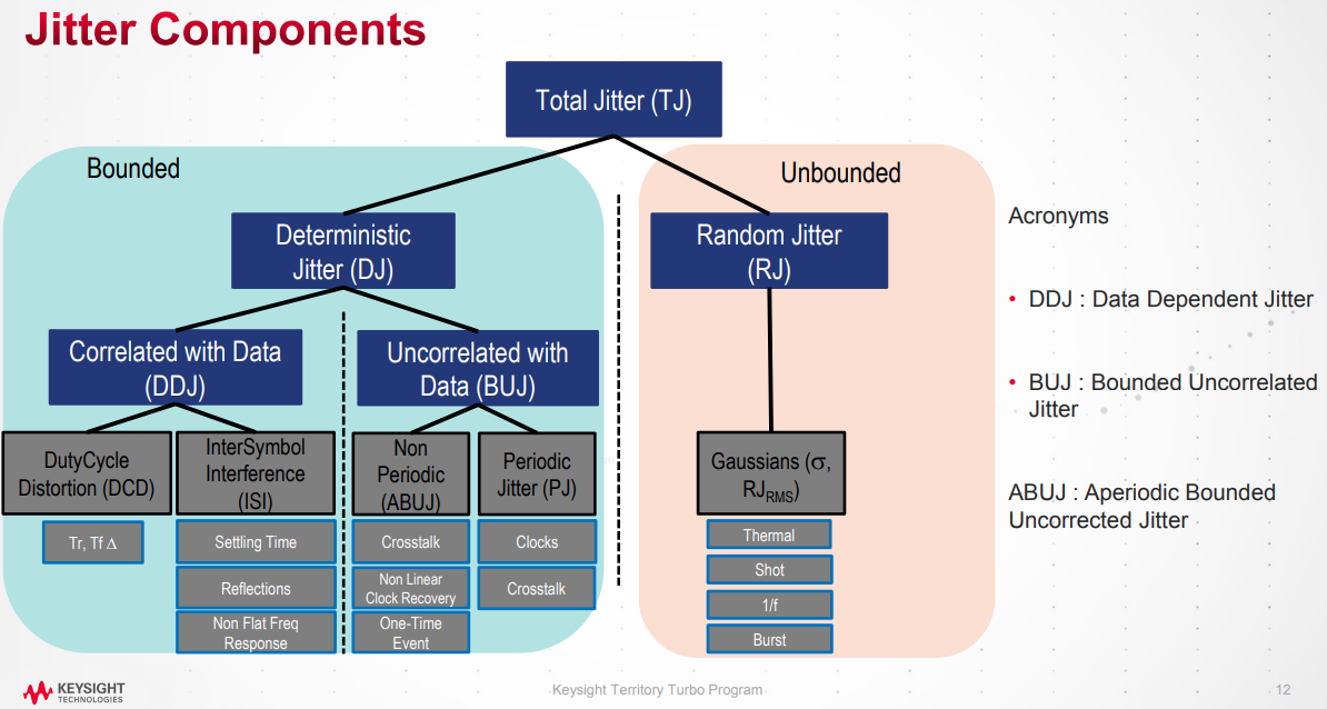
Jitter separation lets you learn if the components of jitter are random or deterministic. That is, if they are caused by crosstalk, channel loss, or some other phenomenon. The identification of jitter and noise sources is critical when debugging failure sources in the transmission of high-speed serial signals
- Tail Fit Method
- Spectral method
| RJ Extraction Methods | Rationale |
|---|---|
| Spectral | Speed/Consistency to Past Measurements; Accuracy in low Crosstalk or Aperiodic Bounded Uncorrelated Jitter (ABUJ) conditions |
| Tail Fit | General Purpose; Accuracy in high Crosstalk or ABUJ conditions |
Jitter Components
dual-Dirac model
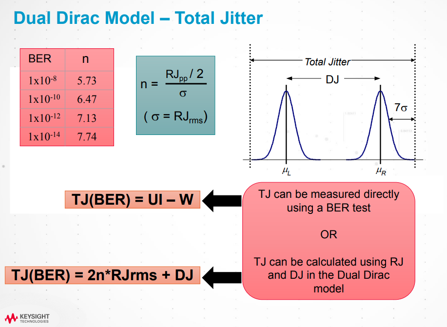
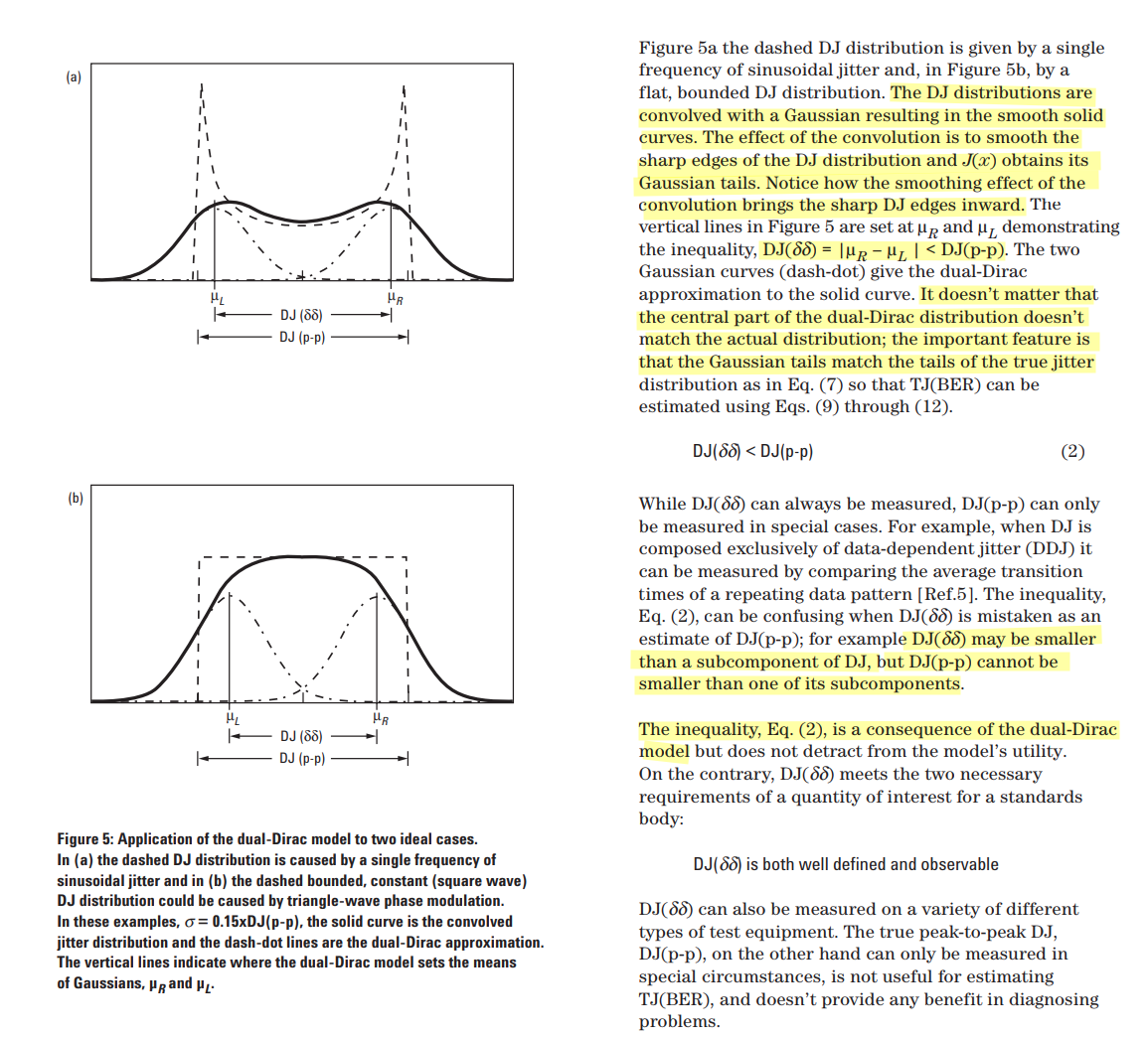
Jitter Analysis: The Dual-Dirac Model, RJ/DJ, and Q-scale [https://people.engr.tamu.edu/spalermo/ecen689/jitter_dual_dirac_agilent.pdf]
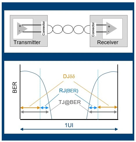
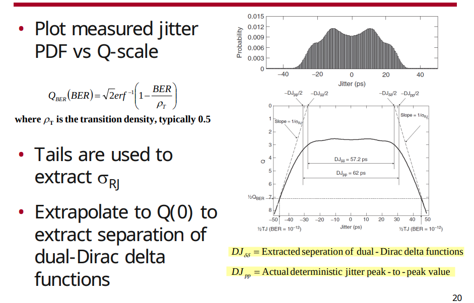
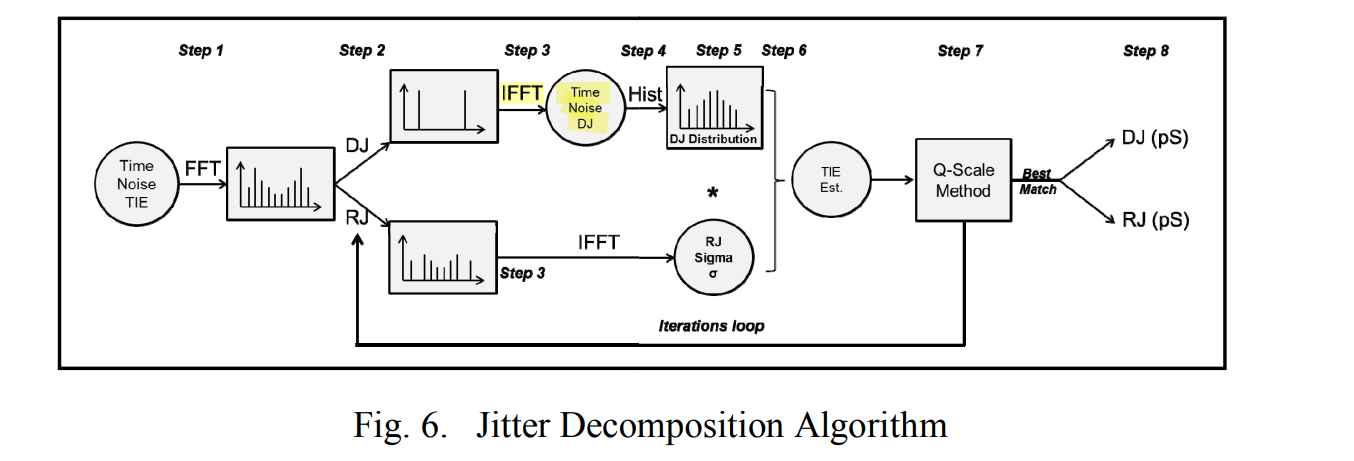
Q-scale
TODO 📅
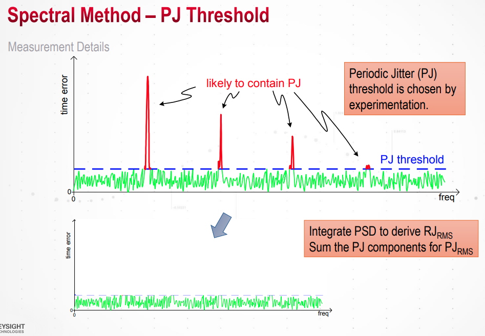
Spectral method
power spectral density (PSD) represents jitter spectrum and peaks in the spectrum can be interpreted as PJ or DDJ, while the average noise floor is the power of RJ
1 | S1 = sum(win); |
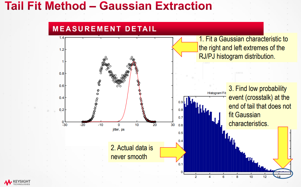
Tail Fit Method
Tail fitting algorithm based on the Gaussian tail model by using probability distribution of collected jitter value
1 | bin_sig = bin_sig*1e12; |
Least Squares (LS) method
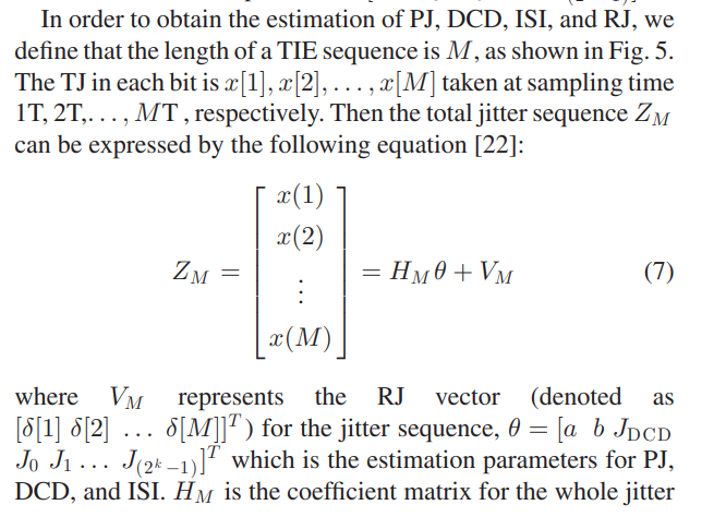
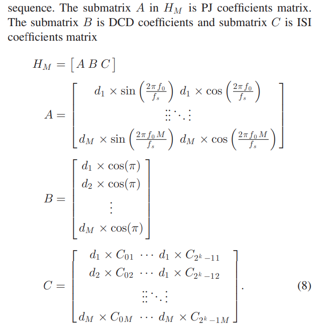
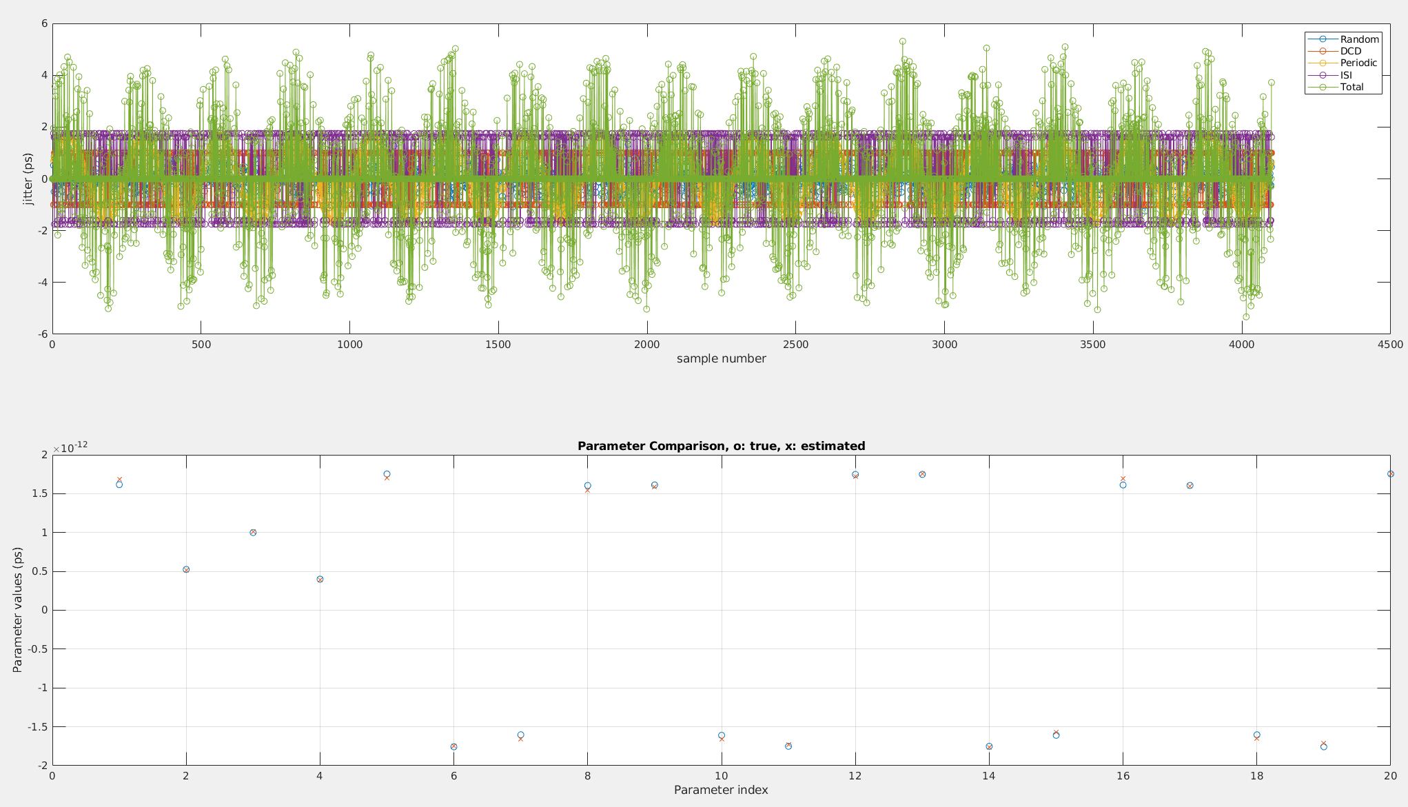
It is known that TIE jitter is a linear equation, shown in below formula \[ x[n] = d_n \times \left[ \Delta t_{pj}[n]+\Delta t_{DCD}[n] +\Delta t_{ISI}[n]+\Delta t_{RJ}[n]\right] \] LS can be used to estimate the PJ, DCD, RJ , and ISI parameters \([a,b,J_{DCD},J_0, J_1...J_{(2^k-1)}]\)
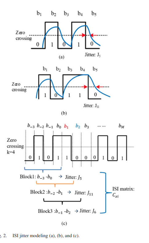
Jitter modeling
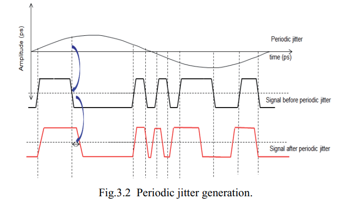
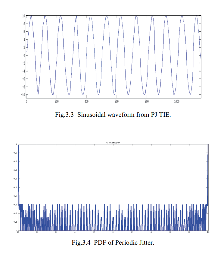
Periodic Jitter (PJ)
PJ is a repeating jitter \[ \Delta t_{PJ}[n]=A\sin(2\pi f_0\cdot nT_s + \theta)=a \sin(2\pi f_0 \cdot nT_s)+b\cos(2\pi f_0 \cdot nT_s) \] where \(f_0\) represents the fundamental frequency of PJ; \(A\) is the amplitude of PJ; \(T_s\) is the data stream period, and \(\theta\) is the initial phase of PJ
In the spectrum, the frequency of maximum amount of the jitter is PJ frequency \(f_0\).
Duty Cycle Distortion (DCD)
DCD is viewed as a series of adjacent positive and negative impulses \[ \Delta t_{DCD}[n] = J_{DCD}\times (-1)^n = [-J_{DCD},J_{DCD},-J_{DCD},J_{DCD},...] \] Where \(J_{DCD}\) is the DCD amplitude.
Random Jitter (RJ)
RJ is created by unbounded jitter sources, such as Gaussian white noise. The statistical PDF for RJ is enerally treated as a Gaussian distribution \[ f_{RJ}(\Delta t) = \frac{1}{\sqrt{2\pi\sigma}}\exp(-\frac{(\Delta t)^2}{2\sigma^2}) \]
DJ/RJ
K. Bidaj, J. -B. Begueret, N. Houdali, J. Deroo and S. Rieubon, "Time-domain PLL modeling and RJ/DJ jitter decomposition," 2016 IEEE International Symposium on Circuits and Systems (ISCAS), Montreal, QC, Canada, 2016 [https://sci-hub.se/10.1109/ISCAS.2016.7527201]
Periodic Jitter Generator & Insertion
Analysis and Estimation of Jitter Sub-Components: Classification and Segregation of Jitter Components
Reference
Li, Mike Peng. Jitter, Noise, and Signal Integrity at High- Speed. Prentice Hall, 2008.
—,DesignCon2007, Simultaneous Jitter Analysis in Time, Frequency, and Statistical Domains and Their Interrelationships [pdf]
—,DesignCon2023, Accuracy and Challenges of PAM4 jitter and noise measurements for >100Gbps Serial Links [pdf]
—, "A new method for jitter decomposition through its distribution tail fitting," International Test Conference 1999. Proceedings (IEEE Cat. No.99CH37034), 1999, pp. 788-794, [https://sci-hub.jp/10.1109/TEST.1999.805809]
余宥浚 Jacky Yu, Keysight Taiwan AEO, Advanced Jitter and Eye-Diagram Analysis
Y. Duan and D. Chen, "Accurate jitter decomposition in high-speed links," 2017 IEEE 35th VLSI Test Symposium (VTS), 2017, pp. 1-6, doi: 10.1109/VTS.2017.7928918.
Y. Duan's phd thesis URL: https://dr.lib.iastate.edu/handle/20.500.12876/30459
Y. Duan and D. Chen, "Fast and Accurate Decomposition of Deterministic Jitter Components in High-Speed Links," in IEEE Transactions on Electromagnetic Compatibility, vol. 61, no. 1, pp. 217-225, Feb. 2019, doi: 10.1109/TEMC.2018.2797122.
"Jitter Analysis: The Dual-Dirac Model, RJ/DJ, and Q-Scale", Whitepaper: Keysight Technologies, U.S.A., Dec. 2017
Sharma, Vijender Kumar and Sujay Deb. "Analysis and Estimation of Jitter Sub-Components." (2014).
Qingqi Dou and J. A. Abraham, "Jitter decomposition in ring oscillators," Asia and South Pacific Conference on Design Automation, 2006
E. Balestrieri, L. De Vito, F. Lamonaca, F. Picariello, S. Rapuano and I. Tudosa, "The jitter measurement ways: The jitter decomposition," in IEEE Instrumentation & Measurement Magazine, vol. 23, no. 7, pp. 3-12, Oct. 2020, doi: 10.1109/MIM.2020.9234759.
McClure, Mark Scott. "Digital jitter measurement and separation." PhD diss., 2005.
Ren, Nan, Zaiming Fu, Shengcu Lei, Hanglin Liu, and Shulin Tian. "Jitter generation model based on timing modulation and cross point calibration for jitter decomposition." Metrology and Measurement Systems 28, no. 1 (2021).
K. Bidaj, J. -B. Begueret and J. Deroo, "RJ/DJ jitter decomposition technique for high speed links," 2016 IEEE International Conference on Electronics, Circuits and Systems (ICECS) [https://sci-hub.se/10.1109/ICECS.2016.7841269]