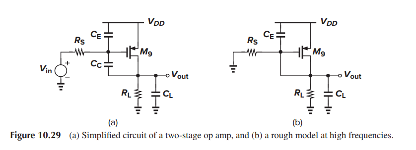
pole splitting

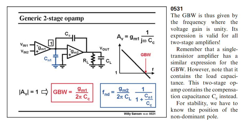
Generic circuit in textbook

In addition to lowering the required capacitor value, Miller compensation entails a very important property: it moves the output pole away from the origin. This effect is called pole splitting

The 1st stage is replaced with Thevenin equivalent circuit , \(V_i \cong V_i \cdot g_{m1}R_{o1}\)

\[\begin{align} \frac{V_i-V_{o1}}{R_{o1}} &= V_{o1}\cdot sC_{o1}+(V_{o1}-V_o)\cdot sC_c \\ V_{o1} &= \frac{V_i+sR_{o1}C_cV_o}{1+sR_{o1}(C_{o1}+C_c)} \end{align}\] \[ (V_{o1}-V_o)sC_c=g_{m2}V_{o1}+V_o(\frac{1}{R_{o2}+sC_L}) \] substitute \(V_{o1}\), we get

\[\begin{align} \frac{V_o}{V_i} &= \frac{(sC_c-g_{m2})R_{o2}}{s^2R_{o1}R_{o2}(C_cC_{o1}+C_LC_{o1}+C_LC_c)+s\left\{ R_{o1}C_c\cdot g_{m2}R_{o2}+R_{o2}(C_c+C_L)+R_{o1}(C_{o1}+C_c) \right\} +1} \\ &= \frac{g_{m2}R_{o2}(s\frac{C_c}{g_{m2}}-1)}{s^2R_{o1}R_{o2}(C_cC_{o1}+C_LC_{o1}+C_LC_c)+s\left\{ R_{o1}C_c\cdot g_{m2}R_{o2}+R_{o2}(C_c+C_L)+R_{o1}(C_{o1}+C_c) \right\} +1} \end{align}\]

left hand plane poles

\[\begin{align} \omega_1 &= \frac{1}{R_{o1}C_c\cdot g_{m2}R_{o2}+R_{o2}(C_c+C_L)+R_{o1}(C_{o1}+C_c)} \\ \omega_2 &= \frac{R_{o1}C_c\cdot g_{m2}R_{o2}+R_{o2}(C_c+C_L)+R_{o1}(C_{o1}+C_c)}{R_{o1}R_{o2}(C_cC_{o1}+C_LC_{o1}+C_LC_c)} \end{align}\]

and RHP (right-hand plane) zero \[ \omega_z=\frac{g_{m2}}{C_c} \]

The circuit with series switch

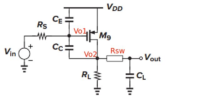
replace \(sC_L\) with \(1/(R_{sw}+\frac{1}{sC_L})\) \[\begin{align} \frac{V_{o2}}{V_i} &= \frac{g_{m2}R_{o2}(s\frac{C_c}{g_{m2}}-1)(1+sR_{sw}C_L)}{s^3R_{o1}R_{o2}R_{sw}C_{o1}C_cC_L+s^2\left\{R_{o1}R_{o2}(C_cC_{o1}+C_LC_{o1}+C_LC_c)+ \left[ R_{o1}C_c\cdot g_{m2}R_{o2}+R_{o2}(C_c+0)+R_{o1}(C_{o1}+C_c)\right]R_{sw}C_L \right\}+s\left\{ R_{o1}C_c\cdot g_{m2}R_{o2}+R_{o2}(C_c+C_L)+R_{o1}(C_{o1}+C_c) +R_{sw}C_L\right\} +1} \end{align}\] Due to \[ \frac{V_o}{V_{o2}} = \frac{\frac{1}{sC_L}}{R_{sw}+\frac{1}{sC_L}}=\frac{1}{1+sR_{sw}C_L} \] Then \[\begin{align} \frac{V_o}{V_i} &= \frac{V_{o2}}{V_i} \cdot \frac{V_o}{V_{o2}} \\ &= \frac{g_{m2}R_{o2}(s\frac{C_c}{g_{m2}}-1)}{s^3R_{o1}R_{o2}R_{sw}C_{o1}C_cC_L+s^2\left\{R_{o1}R_{o2}(C_cC_{o1}+C_LC_{o1}+C_LC_c)+ \left[ R_{o1}C_c\cdot g_{m2}R_{o2}+R_{o2}(C_c+0)+R_{o1}(C_{o1}+C_c)\right]R_{sw}C_L \right\}+s\left\{ R_{o1}C_c\cdot g_{m2}R_{o2}+R_{o2}(C_c+C_L)+R_{o1}(C_{o1}+C_c) +R_{sw}C_L\right\} +1} \end{align}\]

\(R_{sw}\) and \(R_c\)

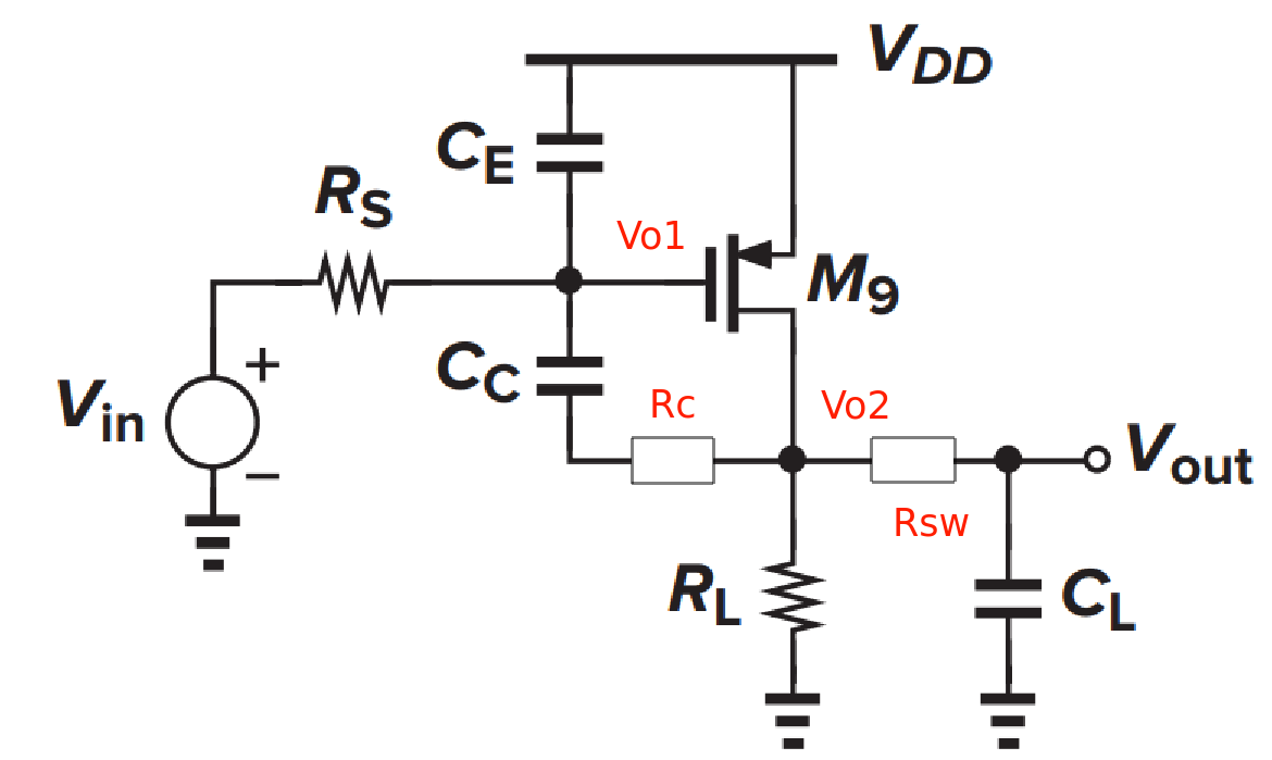
\[\begin{align} \frac{V_{o2}}{V_i} &=-g_{m2}R_{o2}\frac{sC_c(R_c-1/g_{m2})+1}{(1+sR_{o1}C_{o1})sR_{o2}C_c+sR_{o1}\cdot g_{m2}R_{o2}C_c+\frac{s(R_{o2}+R_{sw})C_L+1}{sR_{sw}C_L+1}\left[(1+sR_{o1}C_{o1})(1+sR_cC_c)+sR_{o1}C_c \right]} \\ &=-g_{m2}R_{o2}\frac{sC_c(R_c-1/g_{m2})+1}{s^2R_{o1}R_{o2}C_{o1}C_c+sR_{o2}C_c+sR_{o1}\cdot g_{m2}R_{o2}C_c+\frac{s(R_{o2}+R_{sw})C_L+1}{sR_{sw}C_L+1}\left[(1+sR_{o1}C_{o1})(1+sR_cC_c)+sR_{o1}C_c \right]} \\ &=-g_{m2}R_{o2}\frac{\left[ sC_c(R_c-1/g_{m2})+1 \right](sR_{sw}C_L+1)}{s^2R_{o1}R_{o2}C_{o1}C_c(sR_{sw}C_L+1)+sR_{o2}C_c(sR_{sw}C_L+1)+sR_{o1}\cdot g_{m2}R_{o2}C_c(sR_{sw}C_L+1)+\left[s(R_{o2}+R_{sw})C_L+1\right]\left[(1+sR_{o1}C_{o1})(1+sR_cC_c)+sR_{o1}C_c \right]} \end{align}\]

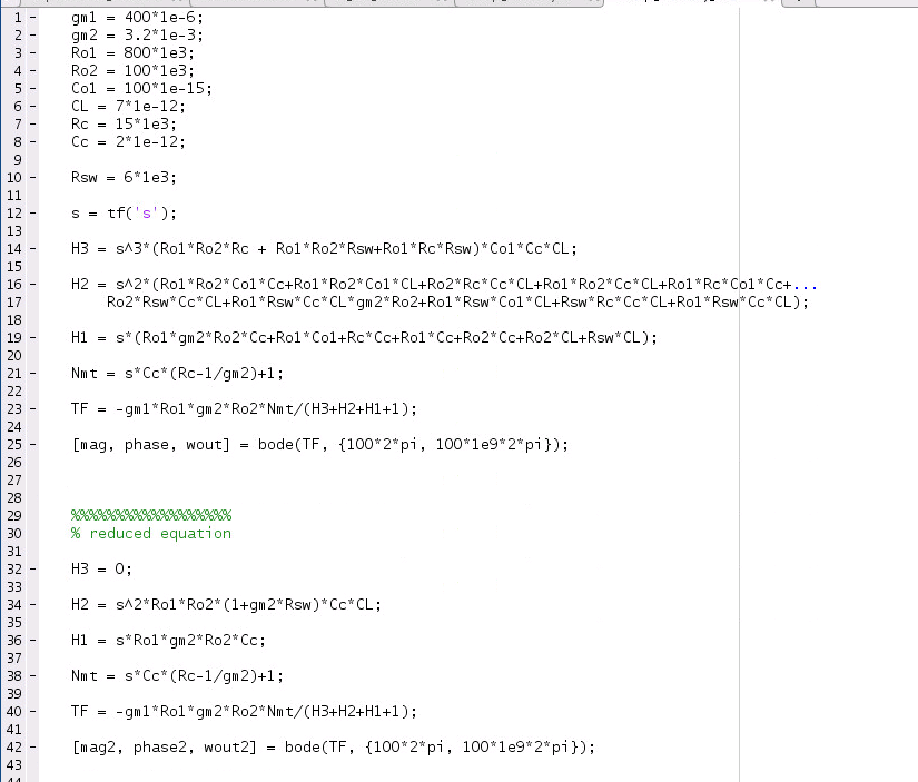
\(s^3\) terms in denominator \[ H_3 = s^3\cdot(R_{o1}R_{o2}R_c+R_{o1}R_{o2}R_{sw} +R_{o1}R_cR_{sw})\cdot C_{o1}C_cC_L \] \(s^2\) terms in denominator \[\begin{align} H_2 &=s^2\cdot(R_{o1}R_{o2}C_{o1}C_c+R_{o1}R_{o2}C_{o1}C_L+R_{o2}R_cC_cC_L+R_{o1}R_{o2}C_cC_L+R_{o1}R_cC_{o1}C_c\\ &+R_{o2}R_{sw}C_cC_L+R_{o1}R_{sw}C_cC_L\cdot g_{m2}R_{o2}+R_{o1}R_{sw}C_{o1}C_L+R_{sw}R_cC_cC_L+R_{o1}R_{sw}C_cC_L) \end{align}\]

\(s^1\) term in denominator \[ H_1=s(R_{o1}\cdot g_{m2}R_{o2}C_c+R_{o1}C_{o1}+R_cC_c+R_{o1}C_c+R_{o2}C_c+R_{o2}C_L+R_{sw}C_L) \] \(s^0\) term in denominator \[ H_0=1 \] set \(R_c=0\) and \(R_{sw}=0\), the \(H_*\) reduced to \[\begin{align} H_3 &= 0 \\ H_2 &=s^2R_{o1}R_{o2}(C_{o1}C_c+C_{o1}C_L+C_cC_L) \\ H_1&=s(R_{o1}\cdot g_{m2}R_{o2}C_c+R_{o1}C_{o1}+R_{o1}C_c+R_{o2}C_c+R_{o2}C_L) \\ H_0&=1 \end{align}\] That is \[ H=s^2R_{o1}R_{o2}(C_{o1}C_c+C_{o1}C_L+C_cC_L)+s(R_{o1}\cdot g_{m2}R_{o2}C_c+R_{o1}C_{o1}+R_{o1}C_c+R_{o2}C_c+R_{o2}C_L)+1 \]

which is same with our previous analysis of Generic circuit in textbook

And we know \[ \frac{V_o}{V_{o2}}=\frac{1}{1+sR_{sw}C_L} \] Finally, we get \(\frac{V_o}{V_i}\) \[\begin{align} \frac{V_o}{V_i} &= \frac{V_{o2}}{V_i} \cdot \frac{V_o}{V_{o2}} \\ &= -g_{m2}R_{o2}\frac{\left[ sC_c(R_c-1/g_{m2})+1 \right](sR_{sw}C_L+1)}{H_3+H_2+H_1+1} \cdot \frac{1}{1+sR_{sw}C_L} \\ &= -g_{m2}R_{o2}\frac{ sC_c(R_c-1/g_{m2})+1}{H_3+H_2+H_1+1} \end{align}\]

The loop transfer function is \[ \frac{V_o}{V_i} =-g_{m1}R_{o1}g_{m2}R_{o2}\frac{ sC_c(R_c-1/g_{m2})+1}{H_3+H_2+H_1+1} \]

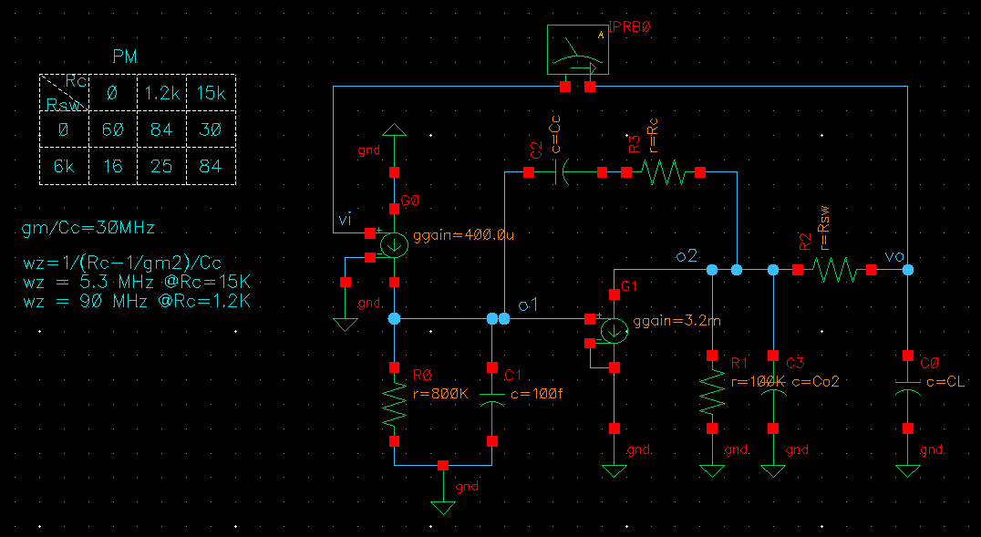
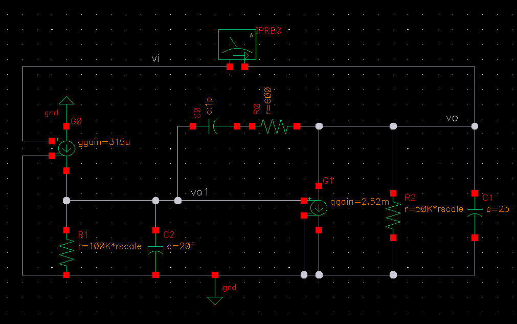
vccs model

simplify the transfer function

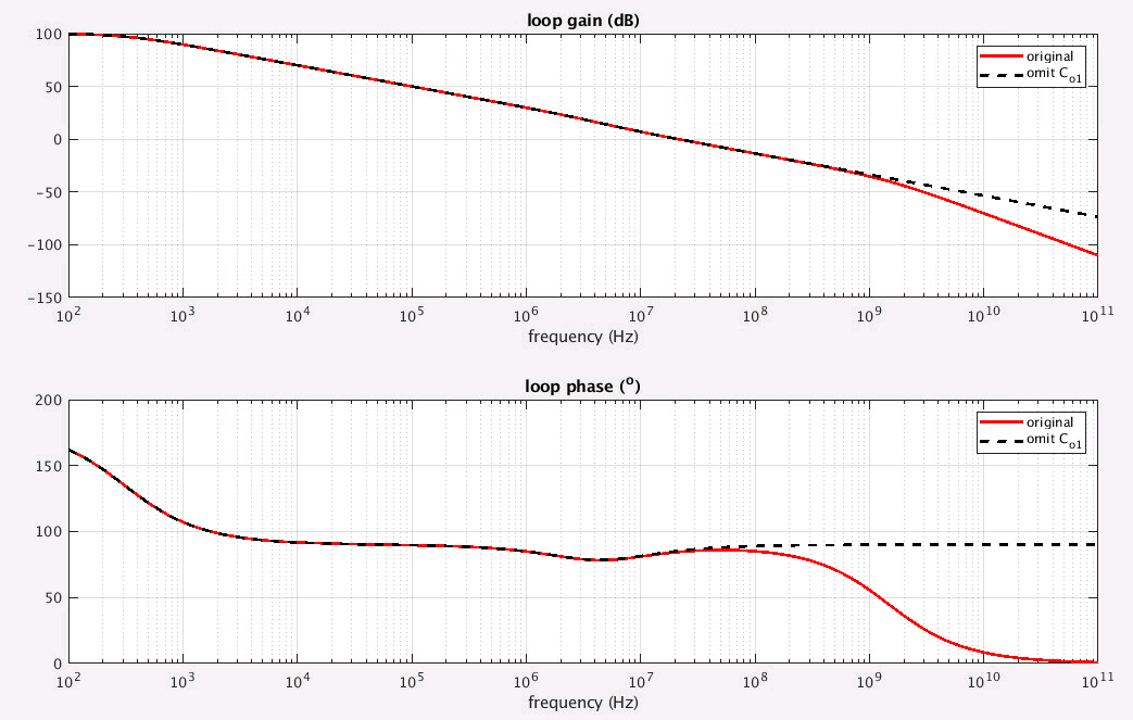
omit \(C_{o1}\)

We omit \(C_{o1}\) in frequency range of interest

\[\begin{align} H_3 &= 0 \\ H_2 &=s^2(R_{o2}R_c+R_{o1}R_{o2}+R_{o2}R_{sw}+R_{o1}R_{sw}\cdot g_{m2}R_{o2}+R_{sw}R_c+R_{o1}R_{sw})\cdot C_cC_L \\ H_1 &=s(R_{o1}\cdot g_{m2}R_{o2}C_c+R_cC_c+R_{o1}C_c+R_{o2}C_c+R_{o2}C_L+R_{sw}C_L) \\ H_0 &= 1 \end{align}\]

two poles and 1 zero

more simplification

Then, some terms can be omitted

\[\begin{align} H_2 &=s^2R_{o1}R_{o2}(1+g_{m2}R_{sw})\cdot C_cC_L \\ H_1 &=sR_{o1}\cdot g_{m2}R_{o2}C_c \\ H_0 &= 1 \end{align}\]

The poles can be deduced \[\begin{align} \omega_1 &= \frac{1}{R_{o1}\cdot g_{m2}R_{o2}C_c} \\ \omega_2 &= \frac{1}{1+g_{m2}R_{sw}}\cdot \frac{g_{m2}}{C_L} \\ &= \frac{1}{(gm_2^{-1}+R_{sw})C_L} \end{align}\]

The pole \(\omega_2=\frac{1}{gm_2^{-1}C_L}\) is changed to \(\omega_2=\frac{1}{(gm_2^{-1}+R_{sw})C_L}\)

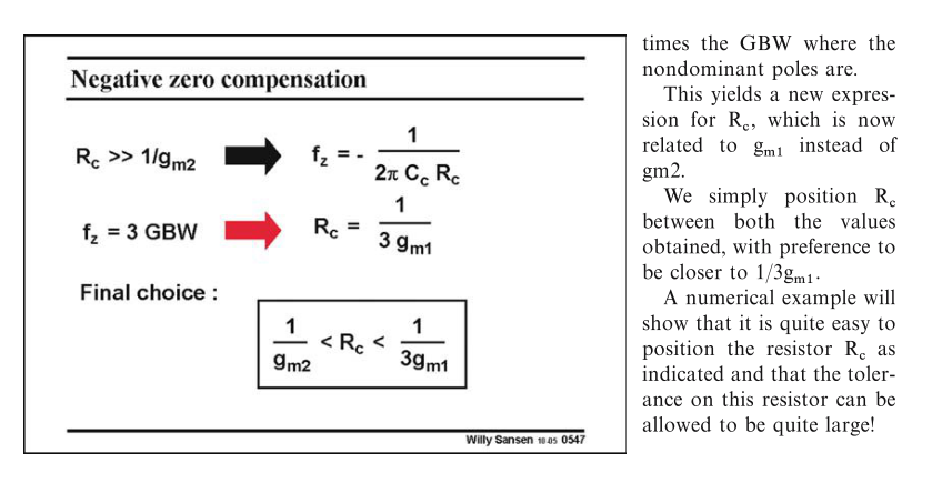
In order to cancell \(\omega_2\) with \(\omega_z\), \(R_c\) shall be increased

\[ R_{eq}=g_{m2}^{-1}+R_{sw} \]

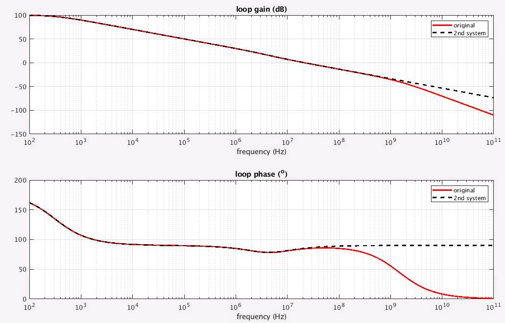
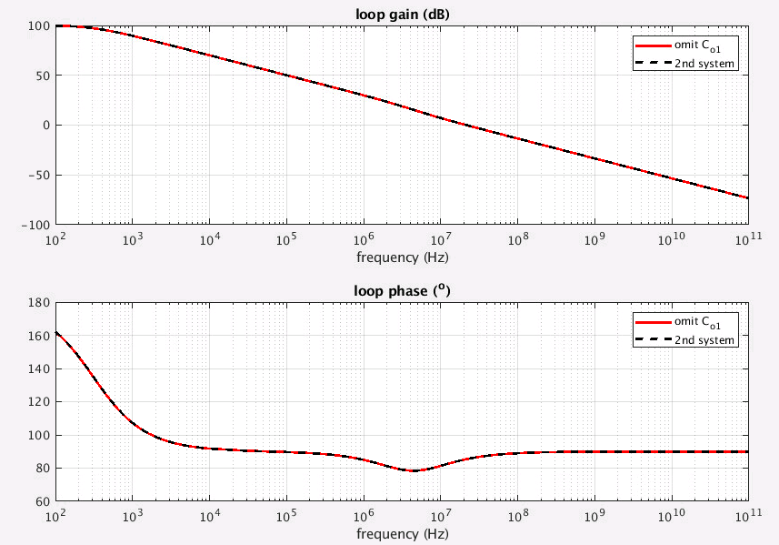
omit \(C_{o1}\) is same with 2nd system simplification

non-dominant pole in Sansen's book

Following demonstrate how derive \(f_{nd}\) from Razavi's equation. We copy \(\omega_2\) here \[ \omega_2 = \frac{R_{o1}C_c\cdot g_{m2}R_{o2}+R_{o2}(C_c+C_L)+R_{o1}(C_{o1}+C_c)}{R_{o1}R_{o2}(C_cC_{o1}+C_LC_{o1}+C_LC_c)} \] which can be reduced as below

\[\begin{align} \omega_2 &= \frac{R_{o1}C_c\cdot g_{m2}R_{o2}+R_{o2}(C_c+C_L)+R_{o1}(C_{o1}+C_c)}{R_{o1}R_{o2}(C_cC_{o1}+C_LC_{o1}+C_LC_c)} \\ &= \frac{R_{o1}C_c\cdot g_{m2}R_{o2}}{R_{o1}R_{o2}(C_cC_{o1}+C_LC_{o1}+C_LC_c)} \\ &= \frac{C_c\cdot g_{m2}}{C_cC_{o1}+C_LC_{o1}+C_LC_c} \\ &= \frac{g_{m2}}{C_{o1}+C_L\frac{C_{o1}}{C_c}+C_L} \\ &= \frac{g_{m2}}{C_L\frac{C_{o1}}{C_c}+C_L} \\ &= \frac{g_{m2}}{C_L} \cdot \frac{1}{1+\frac{C_{o1}}{C_c}} \end{align}\]

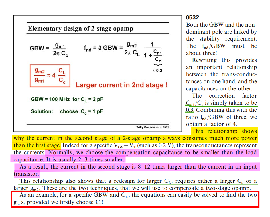
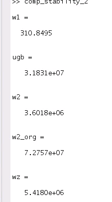
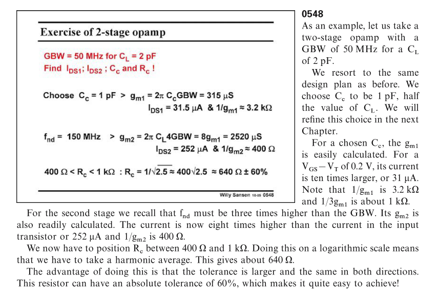
Exercise of 2-stage opamp

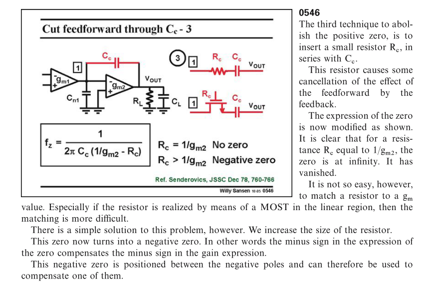
\(R_{o1}\) and \(R_{o2}\) don't affect stability, if \(f_{nd}>3\text{GBW}\)

DC gain: \(g_{m1}g_{m2}R_{o1}R_{o2}\)

dominant pole: \(\omega_d=\frac{1}{R_{o1}\cdot g_{m2}R_{o2}C_c}\)

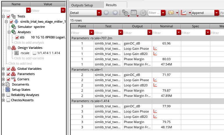
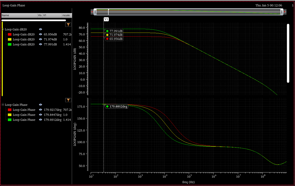
\(20log_{10}(1.414^2)=6\text{dB}\)

reference

Razavi, Behzad. Design of Analog CMOS Integrated Circuits. India: McGraw-Hill, 2017.

Sansen, Willy M. Analog Design Essentials. Germany: Springer US, 2006.