StatEye

Matlab - pulse2stateye

Due to this function only output PDF of eye, postprocessing is needed which cumulative sum PDF.

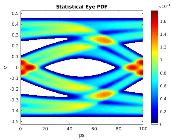
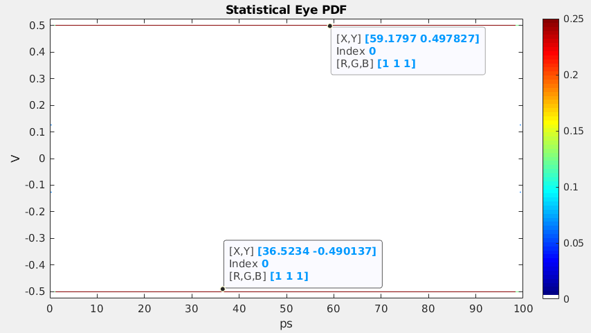
Probability Density Function(PDF) plot

PDF

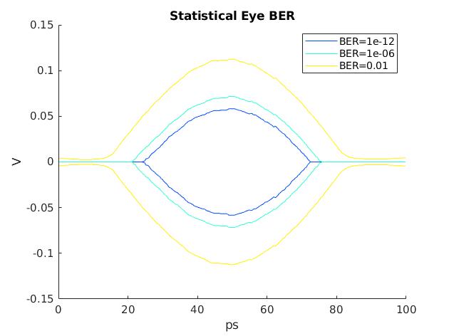
Bit Error Rate(BER) plot
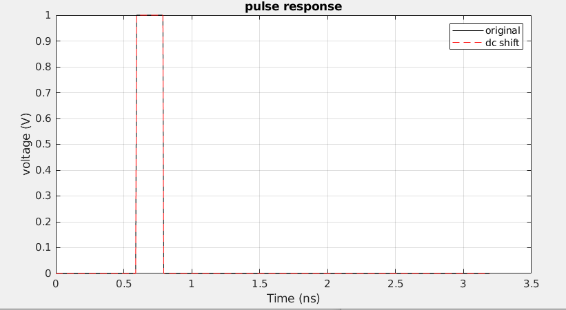
BER

pulse response

image-20220502134522549

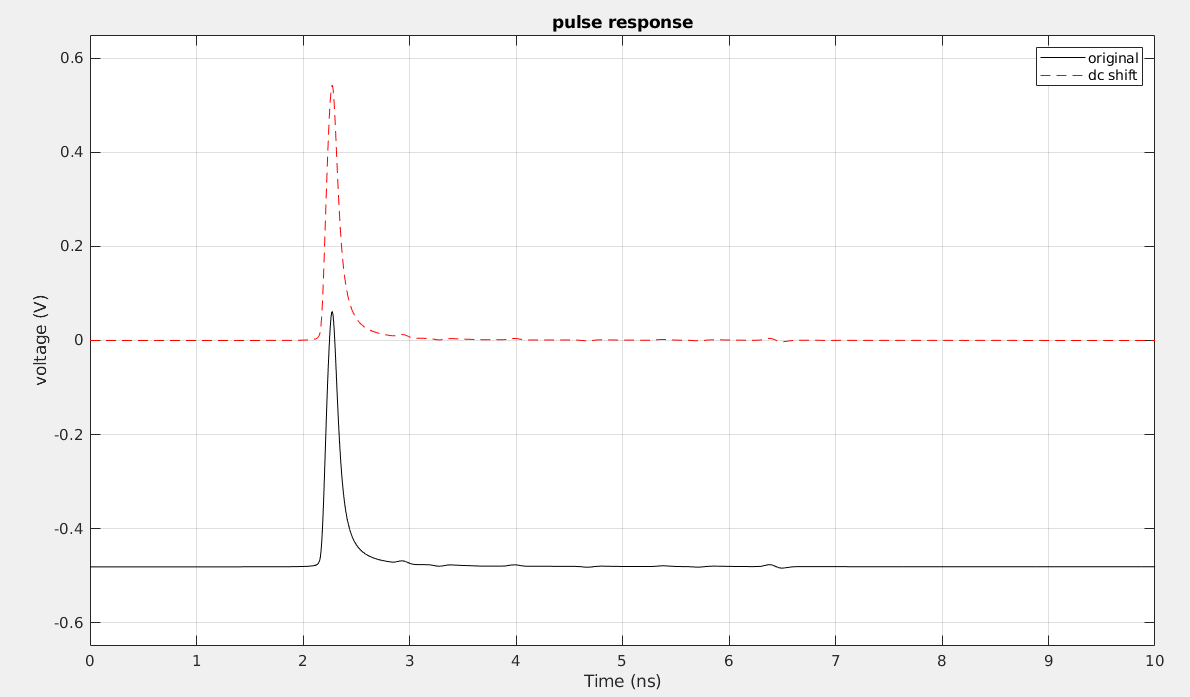
DC shift don't affect pulse2stateye function normally

Both pulse [0 0 0 0 .. 0 1 0 0 0 0 0 ...] and [1 1 1 1 ... 1 0 1 1 1 1 ...] can be fed into

pulse2stateye function

CAUTION: the 0 don't mean common voltage but bit 0 , which is -Vpeak in differential link

postprocessing function

1
2
3
4
5
6
7
8
9
10
11
12
13
14
15
16
17
18
19
20
21
22
23
24
25
26
27
28
29
30
31
32
33
34
35
36
37
38
39
40
41
42
43
44
45
46
47
48
49
50
51
52
53
54
55
56
57
58
59
60
61
62
63
64
65
66
67
68
69
70
71
72
73
74
75
76
77
78
79
80
81
82
83
84
85
86
87
88
89
90
91
92
93
94
95
96
97
98
99
100
101
102
103
104
105
106
107
108
109
110
111
112
113
114
115
116
117
118
119
120
121
122
123
124
125
126
127
128
129
130
131
132
133
134
135
136
137
138
139
140
141
142
% REF: https://www.mathworks.com/help/serdes/ref/pulse2stateye.html
load('PulseResponseReflective100ps.mat');
modulation = 2;
pulsewave = zeros(size(pulse, 1), 1);
pulsewave = pulse(:, 1);
pulsewave(:,1) = pulsewave - pulsewave(1); % DC shift, although `pulse2stateye` shift internally

[stateye,vh,th] = pulse2stateye(pulsewave,SamplesPerSymbol,modulation);
%stateye(1:200, 1:200) = 10000;
cmap = serdes.utilities.SignalIntegrityColorMap;
figure(1);
imagesc(th*SymbolTime*1e12,vh,stateye)
colormap(cmap)
colorbar
axis('xy')
xlabel('ps')
ylabel('V')
title('Statistical Eye PDF')

[ysize, xsize] = size(stateye);
ymid = floor((ysize+1)/2);
upperEyePDF = stateye(ymid:end,:);
lowerEyePDF = stateye(ymid:-1:1,:); % upside down

upperEyeCDF = cumsum(upperEyePDF, 1);
lowerEyeCDF = cumsum(lowerEyePDF, 1);


berlist = [1e-12, 1e-6, 0.01];
lenBer = length(berlist);
upperBERIdx = zeros(lenBer, xsize);
lowerBERIdx = zeros(lenBer, xsize);

for i = 1:lenBer
for j = 1:xsize
upperBERIdx(i, j) = find(upperEyeCDF(:, j) >= berlist(i), 1);
lowerBERIdx(i, j) = find(lowerEyeCDF(:, j) >= berlist(i), 1);
end
end

% shift idx to algin original stateye
upperBERIdx = ymid - 1 + upperBERIdx;
lowerBERIdx = ymid + 1 - lowerBERIdx;

upperBERVal = vh(upperBERIdx);
lowerBERVal = vh(lowerBERIdx);

tticks = th*SymbolTime*1e12;
figure(2);
lgd = cell(lenBer*2,1) ;
hold on;
for i = 1:lenBer% REF: https://www.mathworks.com/help/serdes/ref/pulse2stateye.html
load('PulseResponseReflective100ps.mat');
modulation = 2;
pulsewave = zeros(size(pulse, 1), 1);
pulsewave = pulse(:, 1); % remove crosstalk pulse responses

[stateye,vh,th] = pulse2stateye(pulsewave,SamplesPerSymbol,modulation);
cmap = serdes.utilities.SignalIntegrityColorMap;
figure(1);
imagesc(th*SymbolTime*1e12,vh,stateye)
colormap(cmap)
colorbar
axis('xy')
xlabel('ps')
ylabel('V')
title('Statistical Eye PDF')

[ysize, xsize] = size(stateye);
ymid = floor((ysize+1)/2);
upperEyePDF = stateye(ymid:end,:);
lowerEyePDF = stateye(ymid:-1:1,:); % upside down

upperEyeCDF = cumsum(upperEyePDF, 1);
lowerEyeCDF = cumsum(lowerEyePDF, 1);


berlist = [1e-12, 1e-6, 0.01];
lenBer = length(berlist);
upperBERIdx = zeros(lenBer, xsize);
lowerBERIdx = zeros(lenBer, xsize);

for i = 1:lenBer
for j = 1:xsize
upperBERIdx(i, j) = find(upperEyeCDF(:, j) >= berlist(i), 1);
lowerBERIdx(i, j) = find(lowerEyeCDF(:, j) >= berlist(i), 1);
end
end

% shift idx to algin original stateye
upperBERIdx = ymid - 1 + upperBERIdx;
lowerBERIdx = ymid + 1 - lowerBERIdx;

upperBERVal = vh(upperBERIdx);
lowerBERVal = vh(lowerBERIdx);

tticks = th*SymbolTime*1e12;
figure(2);
lgd = cell(lenBer*2,1) ;
hold on;
for i = 1:lenBer
plot(tticks, upperBERVal(i, :), 'Color', cmap(i*15, :));
lgd{i*2-1} = strcat('BER=',num2str(berlist(i)));
plot(tticks, lowerBERVal(i, :), 'Color', cmap(i*15, :));
lgd{i*2} = "";
end
hold off;
legend(lgd)
axis('xy')
xlabel('ps')
ylabel('V')
title('Statistical Eye BER')

figure(3)
tt = [0:size(pulsewave, 1)-1]*dt;
plot(tt*1e9, pulsewave, 'k', tt*1e9, pulsewave-pulsewave(1), 'r--');
legend('original', 'dc shift');
xlim([0 10]);
ylim([-0.65 0.65])
xlabel('Time (ns)');
ylabel('voltage (V)');
title('pulse response');
grid on;
plot(tticks, upperBERVal(i, :), 'Color', cmap(i*15, :));
lgd{i*2-1} = strcat('BER=',num2str(berlist(i)));
plot(tticks, lowerBERVal(i, :), 'Color', cmap(i*15, :));
lgd{i*2} = "";
end
hold off;
legend(lgd)
axis('xy')
xlabel('ps')
ylabel('V')
title('Statistical Eye BER')

figure(3)
tt = [0:size(pulsewave, 1)-1]*dt;
plot(tt*1e9, pulsewave);
xlabel('Time (ns)');
ylabel('voltage (V)');
title('pulse response');
grid on;

pulse without ISI

Vp2p = 1V

image-20220502135551321

image-20220502135535943

1
2
3
4
5
6
7
8
9
10
11
12
13
14
15
16
17
18
19
20
21
22
23
24
25
modulation = 2;
SamplesPerSymbol = 32;
pulsewave = zeros(SamplesPerSymbol*16, 1);
pulsewave(3*SamplesPerSymbol:4*SamplesPerSymbol-1, 1) = 1;

[stateye,vh,th] = pulse2stateye(pulsewave,SamplesPerSymbol,modulation);
cmap = serdes.utilities.SignalIntegrityColorMap;
figure(1);
imagesc(th*SymbolTime*1e12,vh,stateye)
colormap(cmap)
colorbar
axis('xy')
xlabel('ps')
ylabel('V')
title('Statistical Eye PDF')


figure(2)
tt = [0:size(pulsewave, 1)-1]*dt;
plot(tt*1e9, pulsewave, 'k', tt*1e9, pulsewave-pulsewave(1), 'r--');
legend('original', 'dc shift');
xlabel('Time (ns)');
ylabel('voltage (V)');
title('pulse response');
grid on;

HSPICE - snpsSimADE

use StatEye Analysis in HSPICE

create netlist with hspiceD in Virtuoso
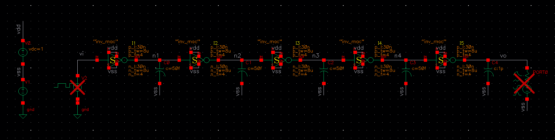
image-20220708011315422

modify netlist

1
2
3
4
5
P1 vi 0  port=1  Z0=0 LFSR (1 0 0 100p 100p 1G 1 [5,2])
P2 vo 0 port=2 Z0=1G
.stateye T=1ns trf=100p incident_port=1 probe_port=2
.probe stateye eye(2) berC(2) eyeBW(2)
.print stateye eye(2) berC(2) eyeBW(2)

Note bothZ0=0 and Z0=1G are used to remove port's effect, which is used as ideal voltage source and voltage monitor
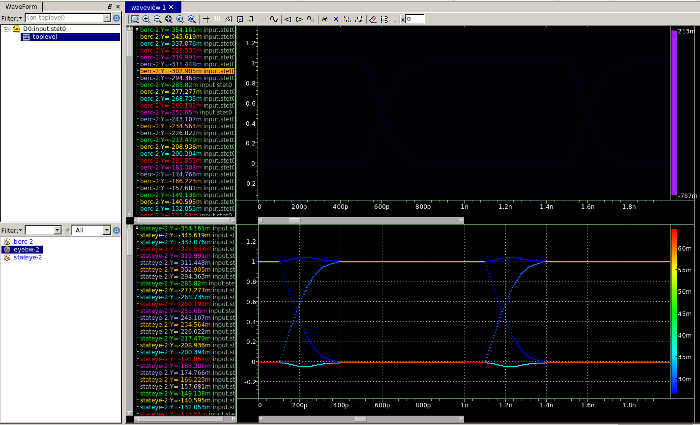
image-20220708012542135

The .probe stateye command generates netlist.stet# and netlist.stev# for following purposes:

  • netlist.stet#: eye(t,v), eyeBW(t,v), eyeV(t), ber(t,v) and bathtubV(t)
  • netlist.stet#: eye(t,v), eyeBW(t,v), eyeV(t), ber(t,v) and bathtubV(t)

setup

.cdsinit

1
load( strcat( getShellEnvVar("HSPICE_HOME") "/hspice/interface/snpsSimADE.ile" ))

environment variable

1
2
export CDS_LOAD_ENV=CSF
export SNPSSIMADE_LOAD_MODE=HSPICE

references

Sanders, Anthony, Michael Resso and John D'Ambrosia. “Channel Compliance Testing Utilizing Novel Statistical Eye Methodology.” (2004).

X. Chu, W. Guo, J. Wang, F. Wu, Y. Luo and Y. Li, "Fast and Accurate Estimation of Statistical Eye Diagram for Nonlinear High-Speed Links," in IEEE Transactions on Very Large Scale Integration (VLSI) Systems, vol. 29, no. 7, pp. 1370-1378, July 2021, doi: 10.1109/TVLSI.2021.3082208.

HSPICE® User Guide: Signal Integrity Modeling and Analysis, Version Q-2020.03, March 2020

IA Title: Common Electrical I/O (CEI) - Electrical and Jitter Interoperability agreements for 6G+ bps, 11G+ bps, 25G+ bps I/O and 56G+ bps IA # OIF-CEI-04.0 December 29, 2017 [pdf]

Chris Li Ph.D. student at the University of Toronto [pystateye repo]