Signal and System insight
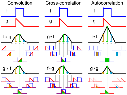
convolution, cross-correlation & autocorrelation
[https://upload.wikimedia.org/wikipedia/commons/2/21/Comparison_convolution_correlation.svg]
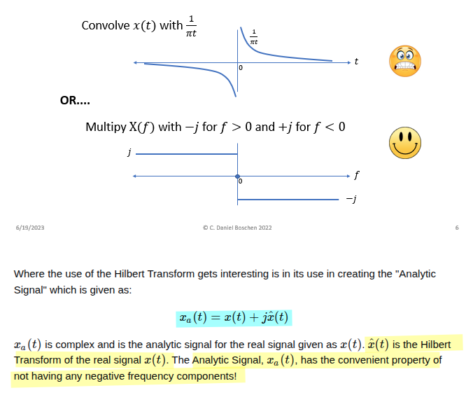
Hilbert Transform
Mathuranathan. Understanding Analytic Signal and Hilbert Transform [https://www.gaussianwaves.com/2017/04/analytic-signal-hilbert-transform-and-fft/]
Dan Boschen. What information does the Hilbert transform give? [https://dsp.stackexchange.com/a/88292/59253]
Frank R. Kschischang. The Hilbert Transform [https://www.comm.utoronto.ca/frank/notes/hilbert.pdf]
Derek Rowell, 2.161 Signal Processing: Continuous and Discrete Fall 2008: Determining a System’s Causality from its Frequency Response [https://ocw.mit.edu/courses/2-161-signal-processing-continuous-and-discrete-fall-2008/142cd928b3b3959721198872ab97b647_causality.pdf]
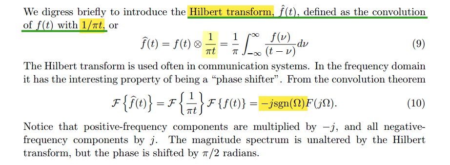
In frequency domain \[ \boxed{\mathcal{H}\{X(\omega)\} = \frac{1}{\pi\omega} * X(\omega)} \qquad \boxed{\mathcal{H}\{x(f)\} = \frac{1}{\pi f} * x(f)} \]
Pulse Amplitude Modulation (PAM)
Qasim Chaudhari. Pulse Amplitude Modulation (PAM) [https://wirelesspi.com/pulse-amplitude-modulation-pam/]
TODO 📅
pulse averaging
The average value of output pulse are same because of same DC gain (0dB)
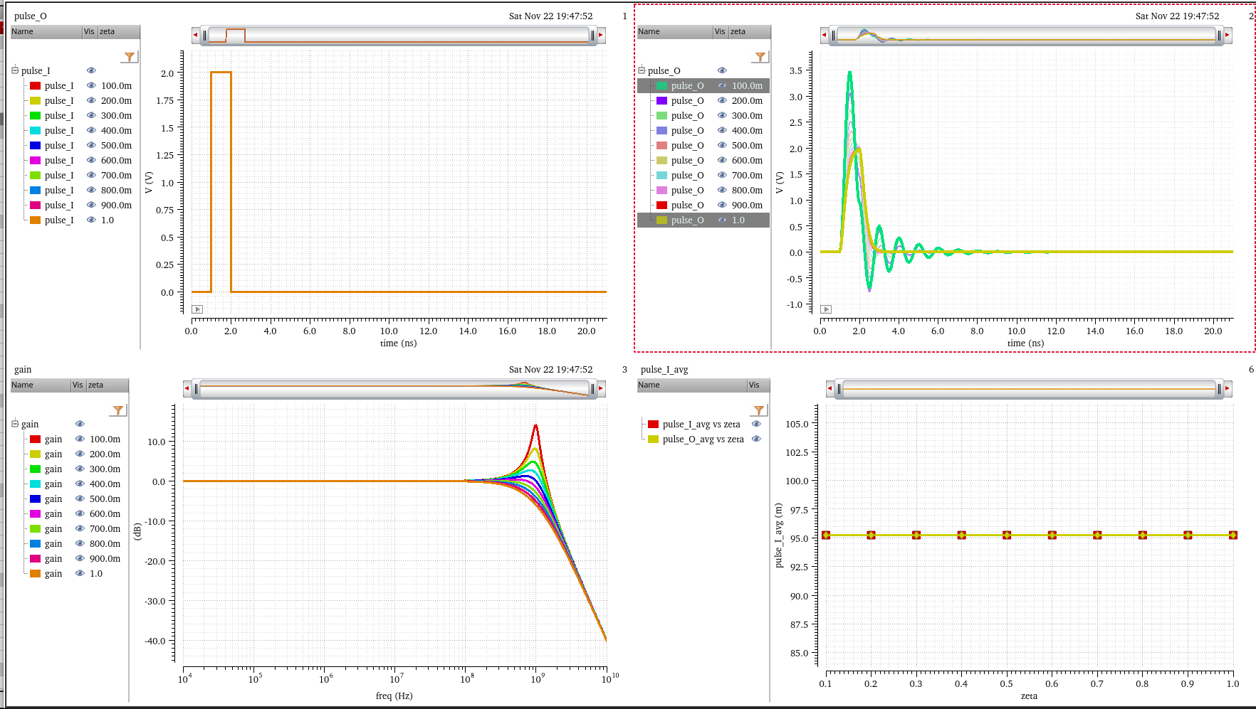
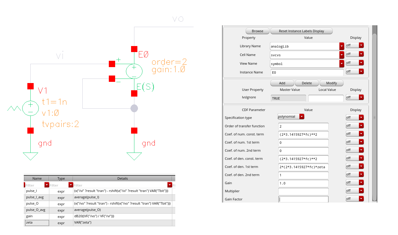
Pulse shape vs Frequency Magnitude
TODO 📅
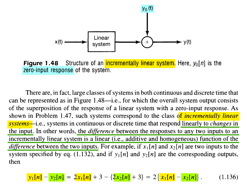
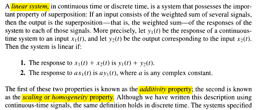
Incrementally linear system
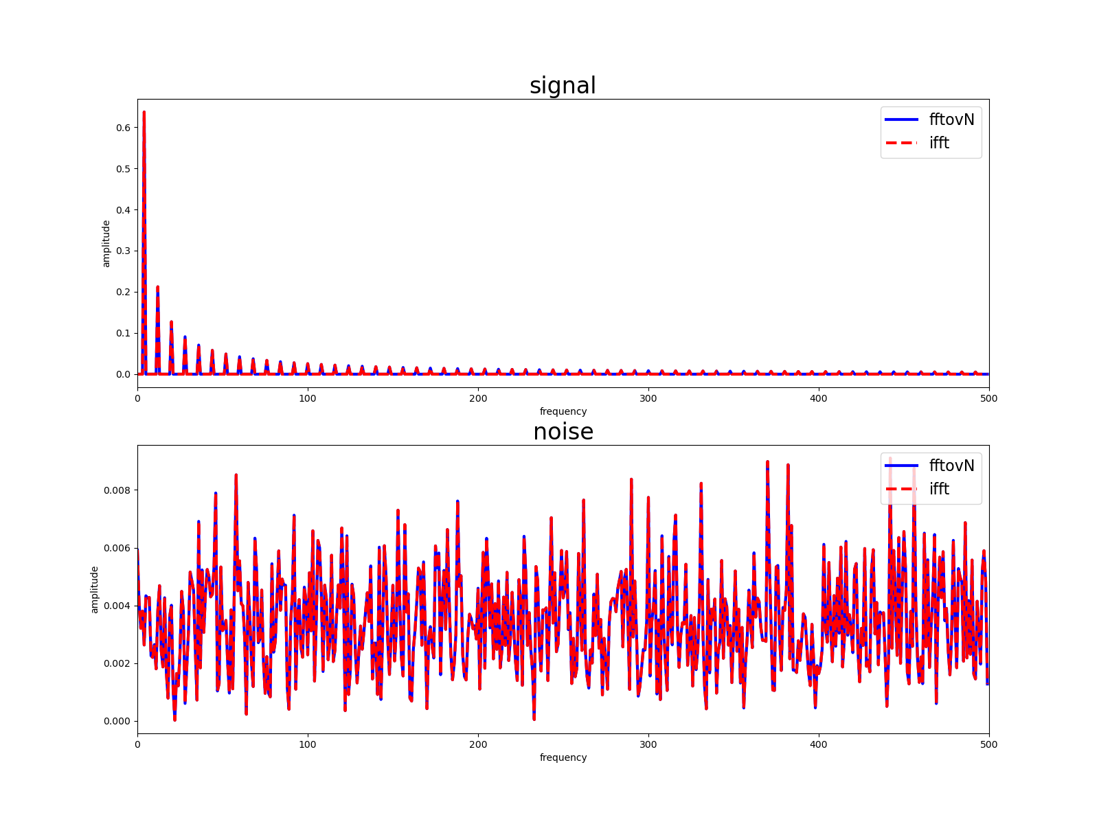
fft vs. ifft
Jason Sachs, Ten Little Algorithms, Part 2: The Single-Pole Low-Pass Filter [https://www.embeddedrelated.com/showarticle/779.php]
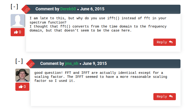
\[
\mathcal{ifft} = \frac{\mathcal{fft}}{N}
\] 
1 | import matplotlib.pyplot as plt |
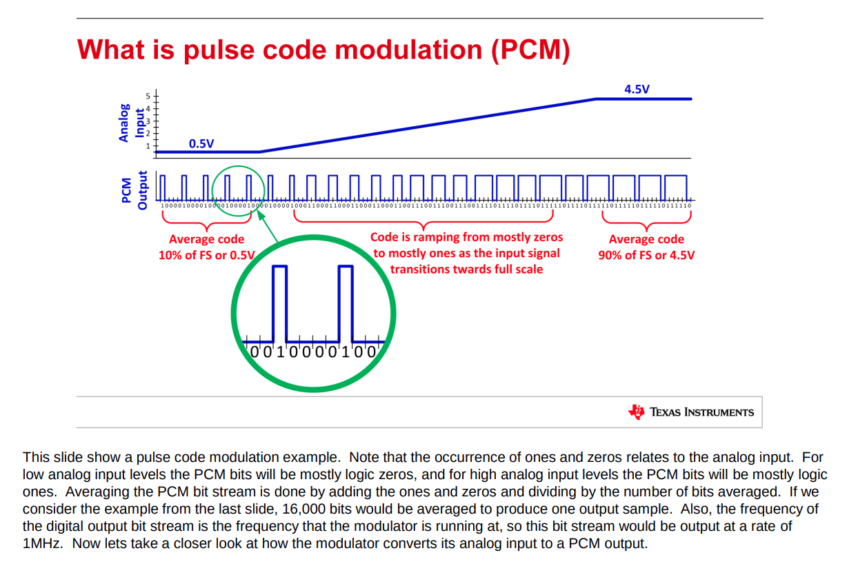
Pulse Code Modulation (PCM)
John M Pauly. Lecture 13: Pulse Code Modulation [https://web.stanford.edu/class/ee179/lectures/notes13.pdf]
Pulse Code Modulation (PCM) is a method for digitally representing analog signals by sampling their amplitude at regular intervals and then encoding these samples into binary numbers
Energy/bit (pJ/b)
1mW/Gbps = 1pJ/bit
Joules are a unit of work or energy. Watts are a unit of power which is the rate at which energy is generated or consumed.
modulation depth
The modulation index (or modulation depth) of a modulation scheme describes by how much the modulated variable of the carrier signal varies around its unmodulated level
TODO 📅
Image frequency
Antonio Liscidini, ESSCIRC 2019 Tutorials: Ultra Low Power Receivers [https://youtu.be/OJRB8g4vUZw]
TODO 📅
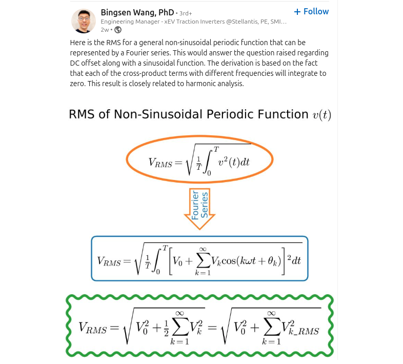
RMS for non-sinusoidal periodic function
Nyquist rate & Nyquist frequency
Nyquist rate
The Nyquist rate is the minimum sample rate required to accurately measure a signal's highest frequency. It's equal to twice the highest frequency of the signal
Nyquist frequency
The Nyquist frequency is the highest frequency that can be represented without aliasing in a discrete signal. It's equal to half the sampling frequency

Oversampling Ratio (OSR) is defined as the ratio of the Nyquist frequency \(f_s/2\) to the signal bandwidth \(B\) given by \(\text{OSR}=f_s/2B\)
Summation & Integration
| impulse response | Transform | ROC | |
|---|---|---|---|
| Summation | \(u(t)\) | \(\frac{1}{s}\) | \(\mathfrak{Re}\{s\}\gt 0\) |
| Integration | \(u[n]\) | \(\frac{1}{1-z^{-1}}\) | \(|z| \gt 1\) |
both are NOT stable
frequency convention
- radian frequency \(\omega_0\) in rad/s
- cyclic frequency \(f_0\) in Hz
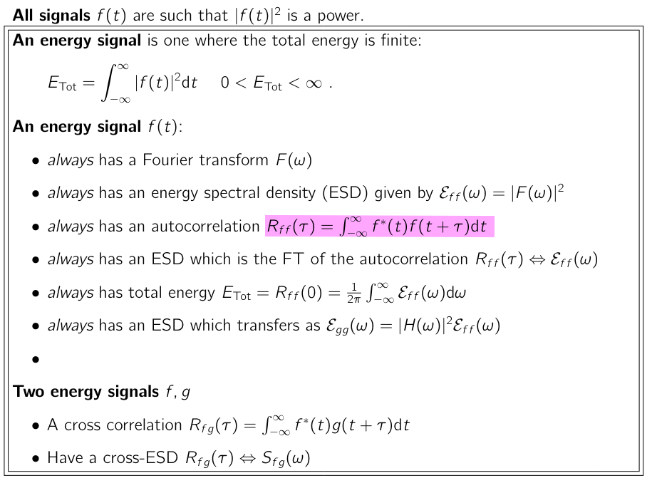
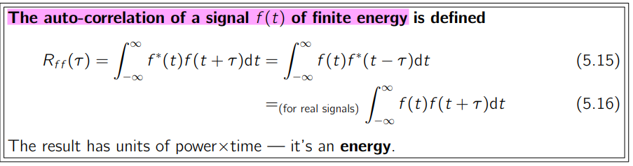
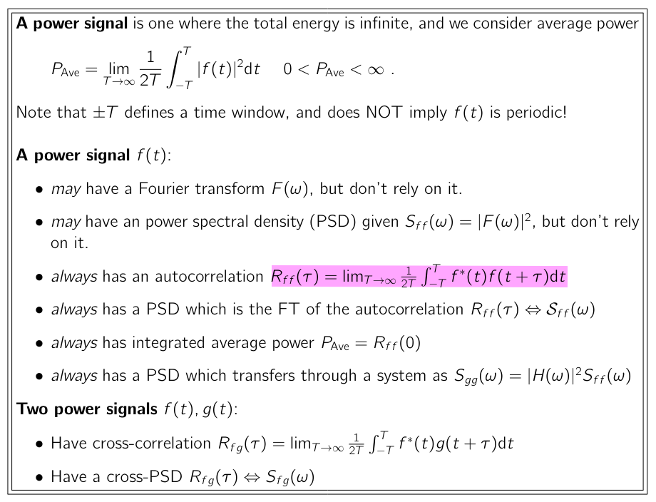
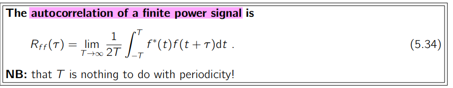
Energy signals vs Power signal
Topic 5 Energy & Power Signals, Correlation & Spectral Density [https://www.robots.ox.ac.uk/~dwm/Courses/2TF_2021/N5.pdf]
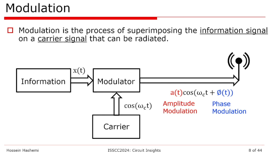
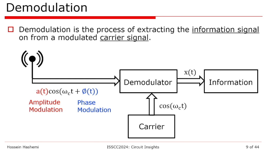
modulation & demodulation
Hossein Hashemi, RF Circuits, [https://youtu.be/0f3yZMvD2Jg]
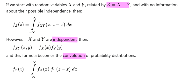
Convolution of probability distributions
The probability distribution of the sum of two or more independent random variables is the convolution of their individual distributions.
Thermal noise
Thermal noise in an ideal resistor is approximately white, meaning that its power spectral density is nearly constant throughout the frequency spectrum.
When limited to a finite bandwidth and viewed in the time domain, thermal noise has a nearly Gaussian amplitude distribution
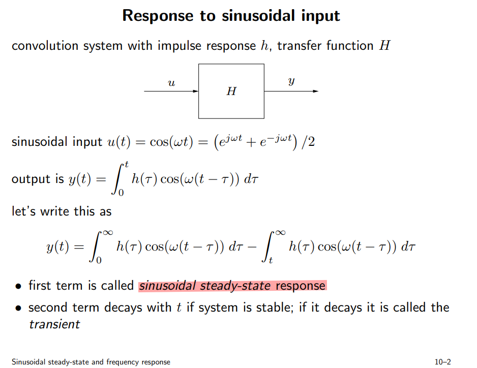
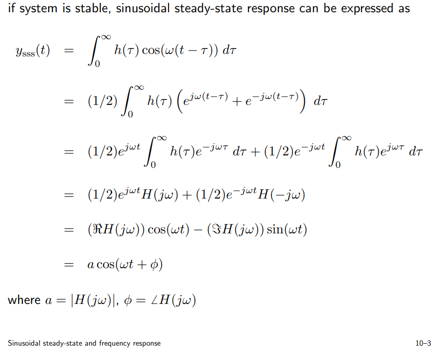
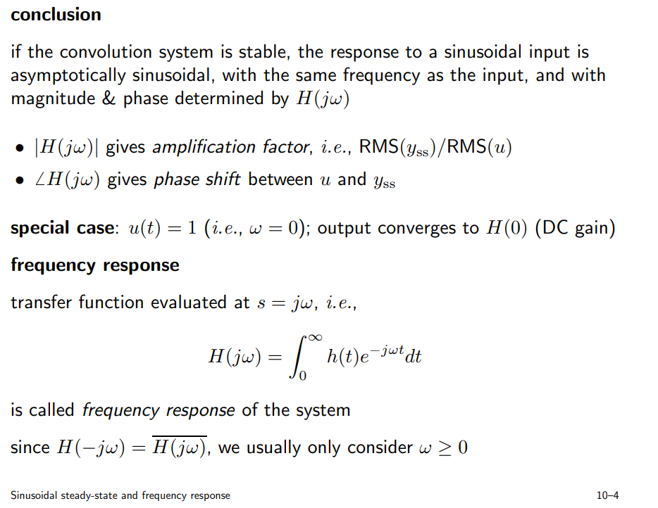
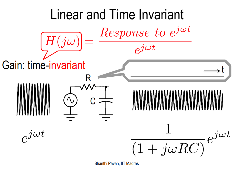
sinusoidal steady-state and frequency response
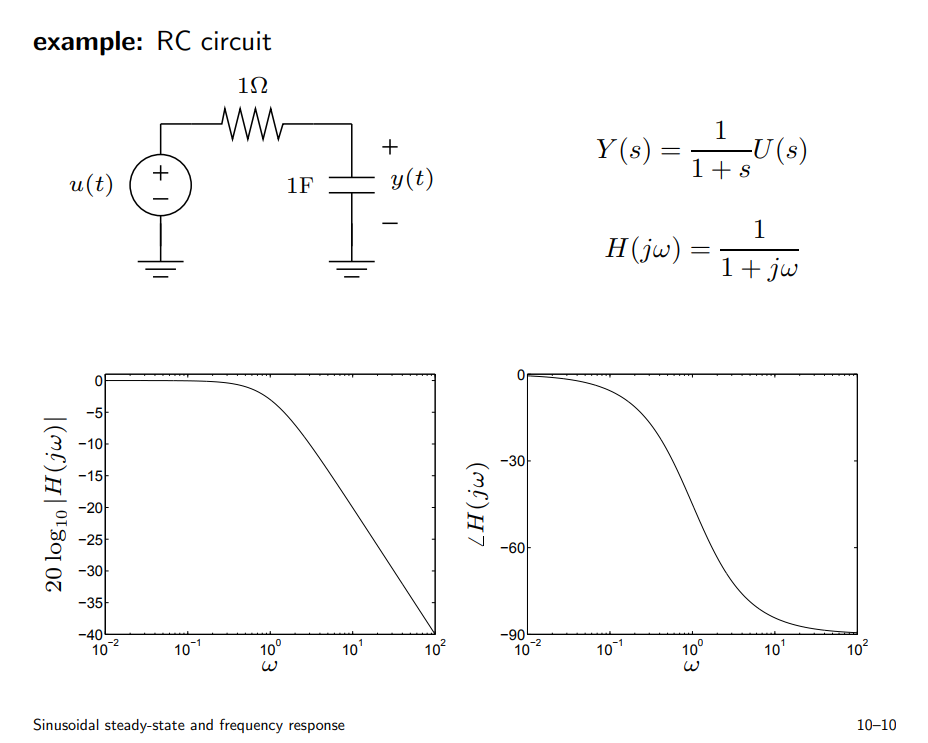
Due to KCL and \(u(t)=e^{j\omega t}\) and \(y(t)=H(j\omega)e^{j\omega t}\), we have ODE:
\[\begin{align} \frac{u(t) - y(t)}{R} = C \frac{\mathrm{d}y(t)}{\mathrm{d}t} \\ e^{j\omega t} - H(j\omega) e^{j\omega t} = H(j\omega)\cdot j\omega e^{j\omega t} \\ \end{align}\]
\(H(j\omega)\) is obtained as below \[ H(j\omega) = \frac{1}{1+j\omega} \]
PSD Definition Variants
In the practice of engineering, it has become customary to use slightly different variants of the PSD definition, depending on the particular application or research field.
Two-Sided PSD, \(S_x(f)\)
this is a synonym of the PSD defined as the Fourier Transform of the autocorrelation.
One-Sided PSD, \(S'_x(f)\)
this is a variant derived from the two-sided PSD by considering only the positive frequency semi-axis.
To conserve the total power, the value of the one-sided PSD is twice that of the two-sided PSD \[ S'_x(f) = \left\{ \begin{array}{cl} 0 & : \ f \geq 0 \\ S_x(f) & : \ f = 0 \\ 2S_x(f) & : \ f \gt 0 \end{array} \right. \]
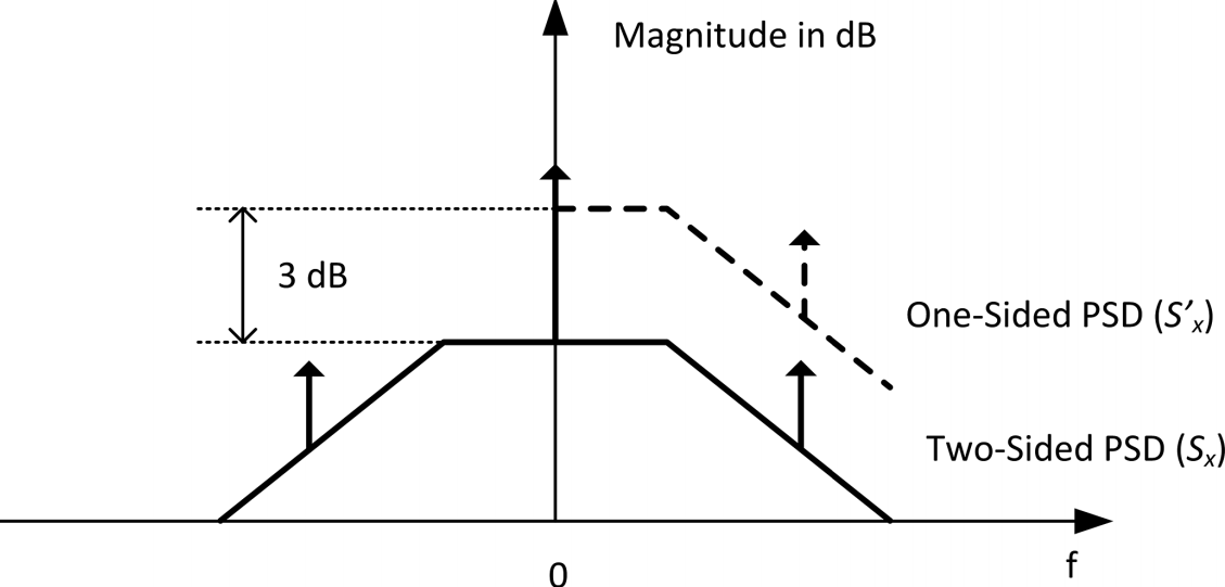
Note that the one-sided PSD definition makes sense only if the two-sided is an even function of \(f\)
If \(S'_x(f)\) is even symmetrical around a positive frequency \(f_0\), then two additional definitions can be adopted:
Single-Sideband PSD, \(S_{SSB,x}(f)\)
This is obtained from \(S'_x(f)\) by moving the origin of the frequency axis to \(f_0\) \[ S_{SSB,x}(f) =S'_x(f+f_0) \] This concept is particularly useful for describing phase or amplitude modulation schemes in wireless communications, where \(f_0\) is the carrier frequency.
Note that there is no difference in the values of the one-sided versus the SSB PSD; it is just a pure translation on the frequency axis.
Double-Sideband PSD, \(S_{DSB,x}(f)\)
this is a variant of the SSB PSD obtained by considering only the positive frequency semi-axis.
As in the case of the one-sided PSD, to conserve total power, the value of the DSB PSD is twice that of the SSB \[ S_{DSB,x}(f) = \left\{ \begin{array}{cl} 0 & : \ f \geq 0 \\ S_{SSB,x}(f) & : \ f = 0 \\ 2S_{SSB,x}(f) & : \ f \gt 0 \end{array} \right. \]
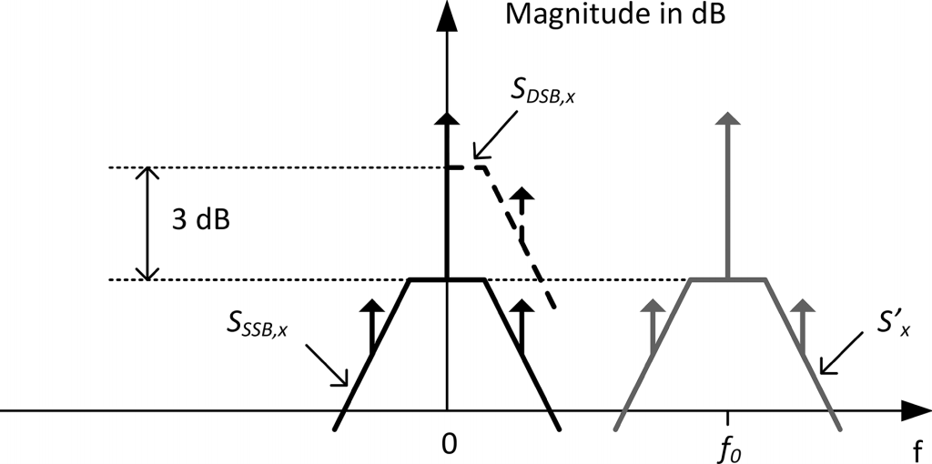
Note that the DSB definition makes sense only if the SSB PSD is even symmetrical around zero
Poles and Zeros of transfer function
poles
\[ H(s) = \frac{1}{1+s/\omega_0} \]
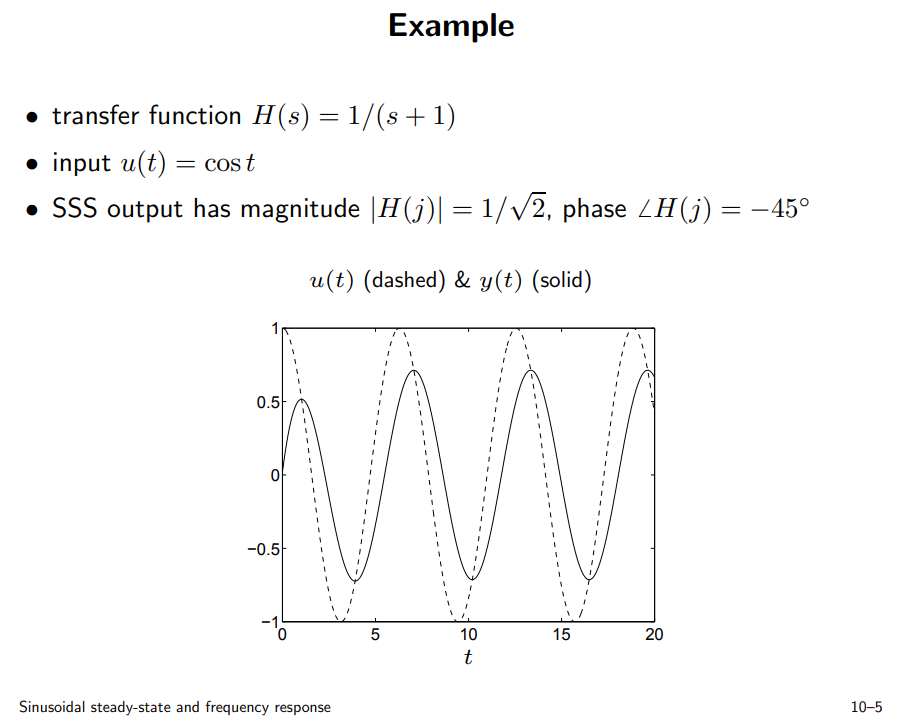
magnitude and phase at \(\omega_0\) and \(-\omega_0\) \[\begin{align} H(j\omega_0) &= \frac{1}{1+j} = \frac{1}{\sqrt{2}}e^{-j\pi/4} \\ H(-j\omega_0) &= \frac{1}{1-j} = \frac{1}{\sqrt{2}}e^{j\pi/4} \end{align}\]
system response \(y(t)\) of input \(\cos(\omega_0 t)\), note \(\cos(\omega_0t) = \frac{1}{2}(e^{j\omega_0 t} + e^{-j\omega_0 t})\) \[\begin{align} y(t) &= H(j\omega_0)\cdot \frac{1}{2}e^{j\omega_0 t} + H(-j\omega_0)\cdot \frac{1}{2}e^{-j\omega_0 t} \\ &= \frac{1}{\sqrt{2}}\cos(\omega_0t-\pi/4) \end{align}\]
\(\cos(\omega_0 t)\), with frequency same with pole DON'T have infinite response
That is, pole indicate decrease trending
zeros
similar with poles, \(\cos(\omega_0 t)\), with frequency same with zero DON'T have zero response
\[ H(s) = 1+s/\omega_0 \]
magnitude and phase at \(\omega_0\) and \(-\omega_0\) \[\begin{align} H(j\omega_0) &= 1+j = \sqrt{2}e^{j\pi/4} \\ H(-j\omega_0) &= 1-j = \sqrt{2}e^{-j\pi/4} \end{align}\]
system response \(y(t)\) of input \(\cos(\omega_0 t)\), note \(\cos(\omega_0t) = \frac{1}{2}(e^{j\omega_0 t} + e^{-j\omega_0 t})\) \[\begin{align} y(t) &= H(j\omega_0)\cdot \frac{1}{2}e^{j\omega_0 t} + H(-j\omega_0)\cdot \frac{1}{2}e^{-j\omega_0 t} \\ &= \sqrt{2}\cos(\omega_0t+\pi/4) \end{align}\]
baud rate
symbol rate, modulation rate or baud rate is the number of symbol changes per unit of time.
- Bit rate refers to the number of bits transmitted between two devices per unit of time
- The baud or symbol rate refers to the number of symbols that can be sent in the same amount of time
reference
Stephen P. Boyd. EE102 Lecture 10 Sinusoidal steady-state and frequency response [https://web.stanford.edu/~boyd/ee102/freq.pdf]
Gene F. Franklin, J. David Powell, and Abbas Emami-Naeini. 2018. Feedback Control of Dynamic Systems (8th Edition) (8th. ed.). Pearson.
Inter-Symbol Interference (or Leaky Bits) [http://blog.teledynelecroy.com/2018/06/inter-symbol-interference-or-leaky-bits.html]
[AN001] Designing from zero an IIR filter in Verilog using biquad structure and bilinear discretization. URL:[https://www.controlpaths.com/articles/an001_designing_iir_biquad_filter_bilinear/]
Frequency warping using the bilinear transform. URL:[https://www.controlpaths.com/2022/05/09/frequency-warping-using-the-bilinear-transform/]
Digital control loops. Theoretical approach. URL:[https://www.controlpaths.com/2022/02/28/digital-control-loops-theoretical-approach/]
Simulation of DSP algorithms in Verilog. URL:[https://www.controlpaths.com/2023/05/20/simulation-of-dsp-algorithms-in-verilog/]
Implementing a digital biquad filter in Verilog. URL:[https://www.controlpaths.com/2021/04/19/implementing-a-digital-biquad-filter-in-verilog/]
Implementing a FIR filter using folding. URL:[https://www.controlpaths.com/2021/05/17/implementing-a-fir-filter-using-folding/]
Oppenheim, Alan V. and Cram. “Discrete-time signal processing : Alan V. Oppenheim, 3rd edition.” (2011).
Extras: PID Compensator with Bilinear Approximation URL:[https://ctms.engin.umich.edu/CTMS/index.php?aux=Extras_PIDbilin]