Data Converter
Quantization Noise
Quantization Error

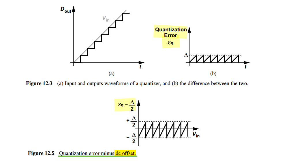
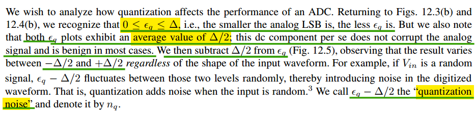
Notice \(e_q\in (0, \Delta)\) and its average is \(\Delta/2\). To calculate SNDR, DC component shall be excluded
Don't confuse resolution \(\Delta\) with Bounded Quantization Noise \(-\Delta/2 \sim \Delta/2\)
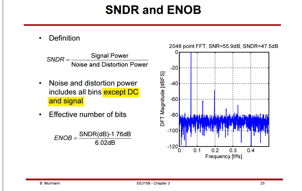
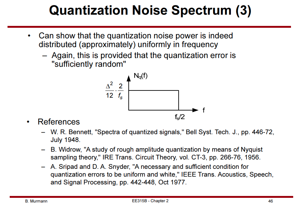
Quantization Noise Spectrum
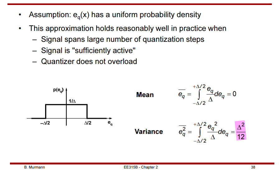
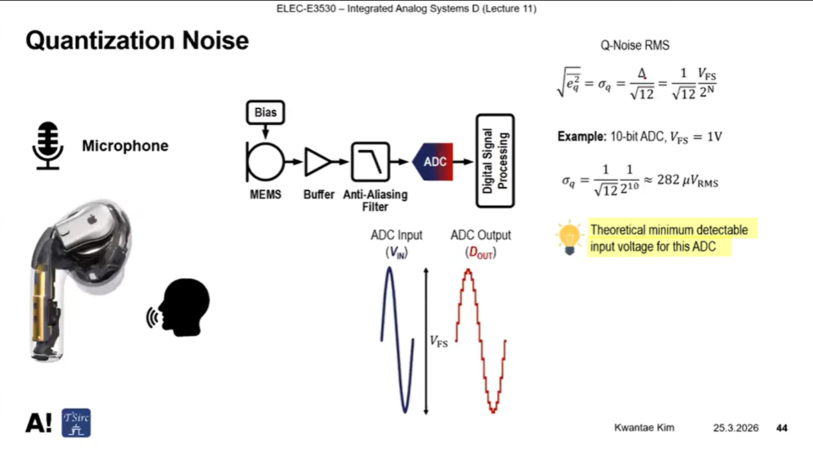
Quantization noise is less with higher resolution as the input range is divided into a greater number of smaller ranges
This error can be considered a quantization noise with RMS
ADC Input Noise
Walt Kester, ADC Input Noise: The Good, The Bad, and The Ugly. Is No Noise Good Noise? [link] [pdf]
—, MT-004: The Good, the Bad, and the Ugly Aspects of ADC Input Noise-Is No Noise Good Noise? [https://www.analog.com/media/en/training-seminars/tutorials/mt-004.pdf]
Understanding ADC Noise for Small and Large Signal Inputs for Receiver Applications [https://www.analog.com/en/resources/technical-articles/understanding-adc-noise-for-small-and-large-signal-inputs-for-receiver-applications.html]
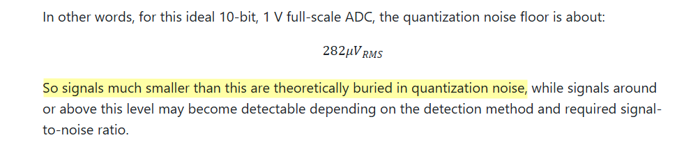
The LSB determines the ADC code resolution, but the minimum reliably detectable input voltage is determined by the total noise floor, including quantization noise
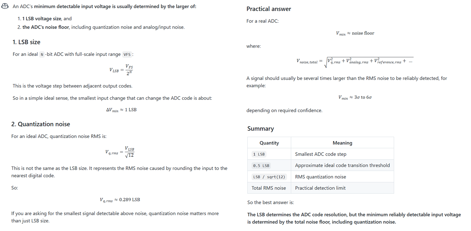
[https://share.google/aimode/aA1V4uj3GofKbBojl]
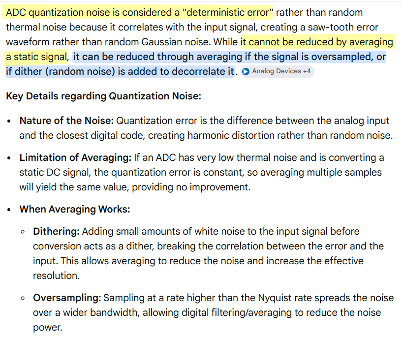
ADC quantization noise is considered a "deterministic error" rather than random thermal noise because it correlates with the input signal, creating a saw-tooth error waveform rather than random Gaussian noise. While it cannot be reduced by averaging a static signal, it can be reduced through averaging if the signal is oversampled, or if dither (random noise) is added to decorrelate it.
Quantization is NOT Noise
N. Blachman, "The intermodulation and distortion due to quantization of sinusoids," in IEEE Transactions on Acoustics, Speech, and Signal Processing, vol. 33, no. 6, pp. 1417-1426, December 1985 [https://sci-hub.st/10.1109/TASSP.1985.1164729]
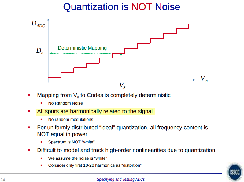
Carsten Wulff, Oversampling and Sigma-Delta ADCs [https://analogicus.com/aic2026/oversampling_and_sigma-delta_adcs] [video] [slides]
N. Blachman, "The intermodulation and distortion due to quantization of sinusoids," in IEEE Transactions on Acoustics, Speech, and Signal Processing, vol. 33, no. 6, pp. 1417-1426, December 1985
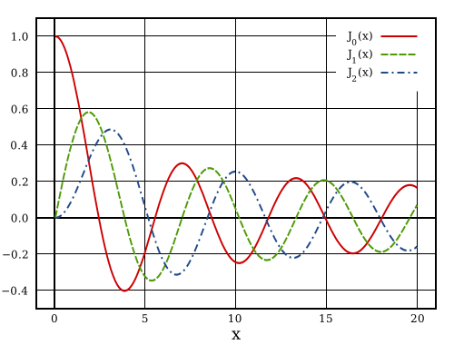
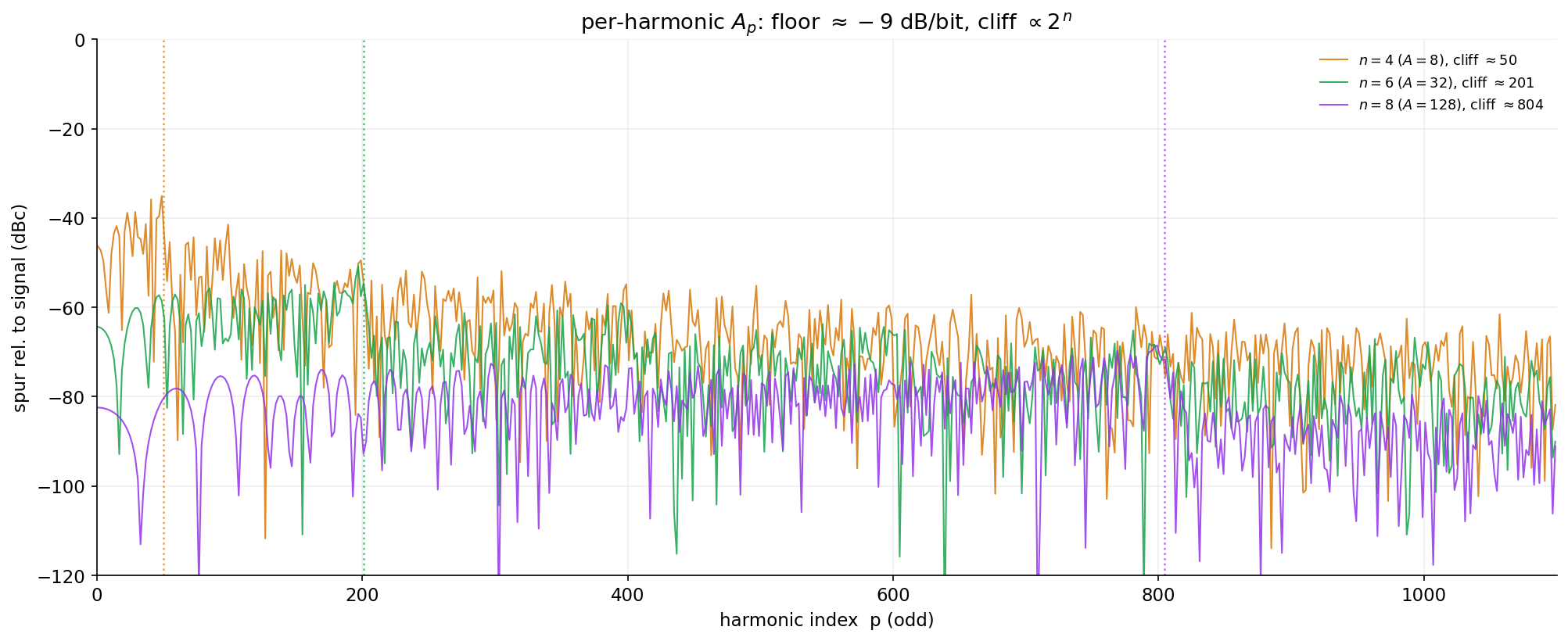
The quantization noise is an infinite sum of input signal odd harmonics, where the amplitude of the harmonics is determined by a sum of a Bessel function
"Quantization noise is white", because for a high number of bits, it looks white in the FFT
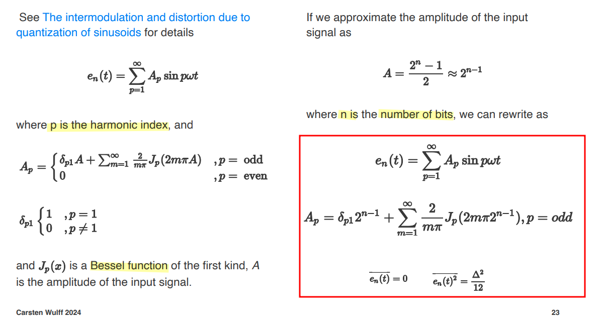
The quantization noise is odd harmonics of the input signal [Gist link]
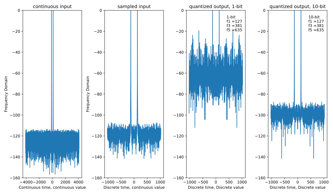
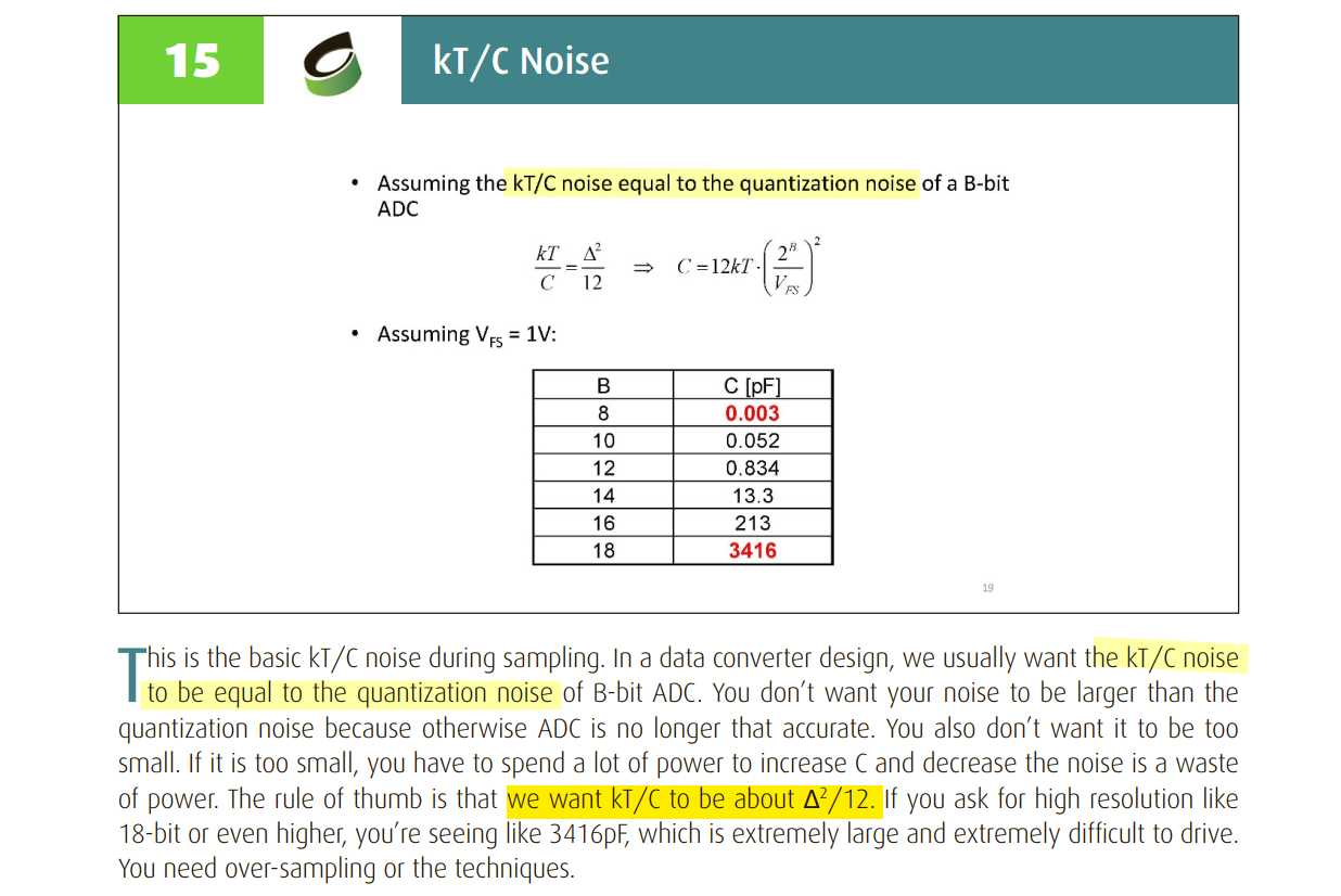
Sampling Noise in ADC
Kwantae Kim, Integrated Analog Systems D - Lecture 12 (ADC) [https://youtu.be/NkSitVkPNig]
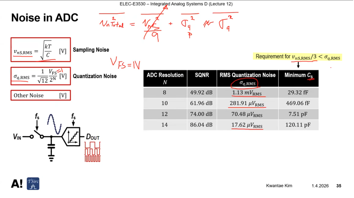
In the power domain, \(\color{red}v_{nS,RMS}/3 \lt \sigma_{q,RMS}\) ensures that sampling noise power is nearly an order of magnitude smaller than the quantization noise
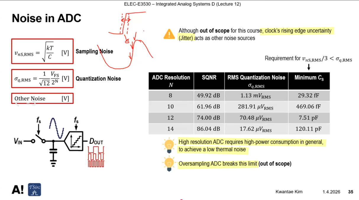
ADC SNR & clock jitter
Akkaya, A. (2021). High-Speed ADC Design and Optimization for Wireline Links (Publication No. 8453) [PhD thesis, EPFL; Supervised by Y. Leblebici]. [https://doi.org/10.5075/epfl-thesis-8453]
CC Chen, Why Absolute Jitter Matters for ADCs & DACs? [https://youtu.be/jBgDDFFDq30]
Thomas Neu, TIPL 4704. Jitter vs SNR for ADCs [https://www.ti.com/content/dam/videos/external-videos/en-us/2/3816841626001/5529003238001.mp4/subassets/TIPL-4704-Jitter-vs-SNR.pdf]
Walt Kester , MT-007: Aperture Time, Aperture Jitter, Aperture Delay Time [https://www.analog.com/media/en/training-seminars/tutorials/MT-007.pdf]
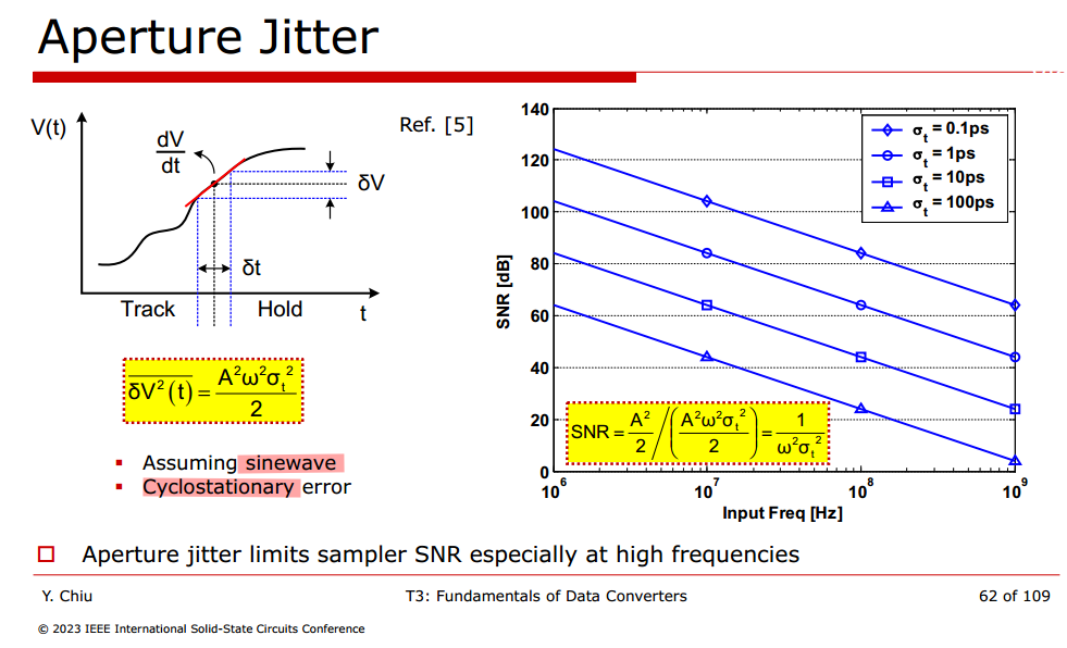
cyclostationary random process
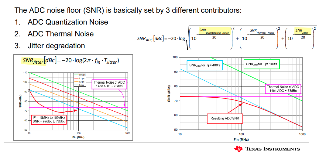
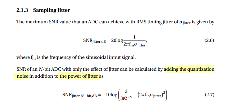
\[\begin{align} \text{SNR}_\text{ADC}[\text{dB}] &= -20\cdot \log \sqrt{\left(10^{-\frac{\text{SNR}_\text{Quantization Noise}}{20}}\right)^2 + \left(10^{-\frac{\text{SNR}_\text{Jitter}}{20}}\right)^2} \\ &= -10\cdot \log \left(\left(10^{-\frac{\text{SNR}_\text{Quantization Noise}}{20}}\right)^2 + \left(10^{-\frac{\text{SNR}_\text{Jitter}}{20}}\right)^2\right) \\ &= -10\cdot \log \left(\left(10^{-\frac{10\log(\frac{3\times2^{2N}}{2})}{20}}\right)^2 + \left(10^{-\frac{-20\log{(2\pi f_\text{in}\sigma_\text{jitter})}}{20}}\right)^2\right) \\ &= -10\cdot \log \left( \frac{2}{3\times 2^{2N}} + (2\pi f_\text{in}\sigma_\text{jitter})^2 \right) \end{align}\]
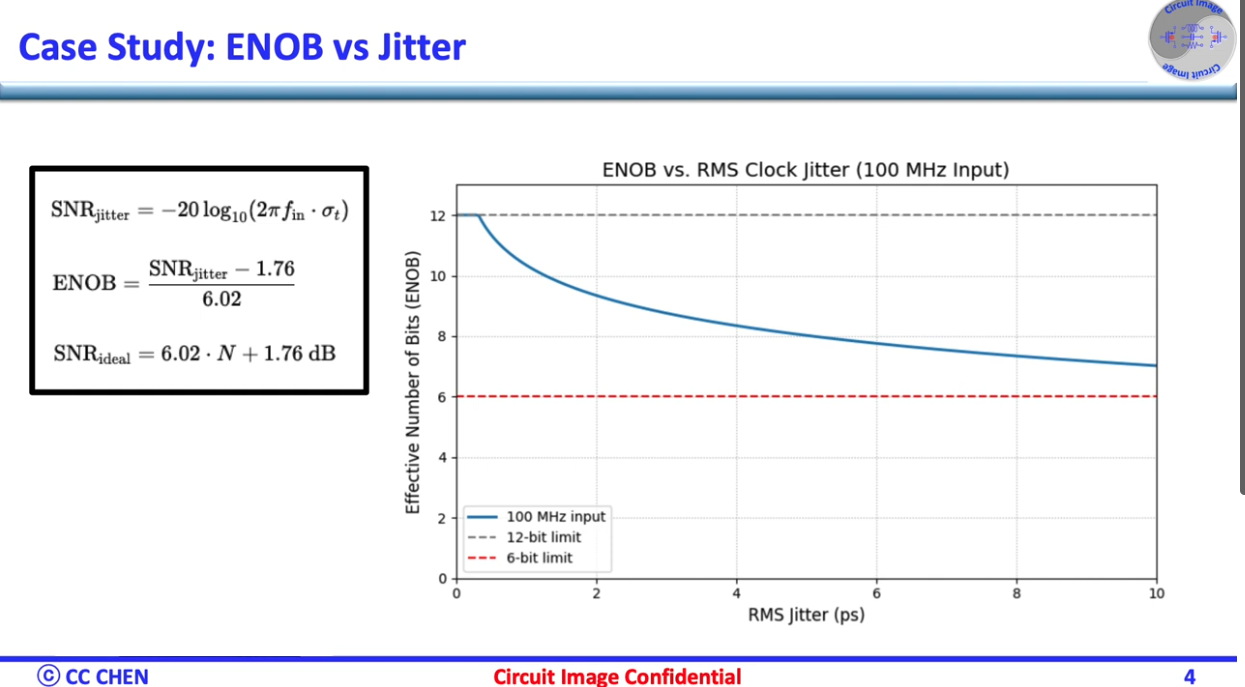
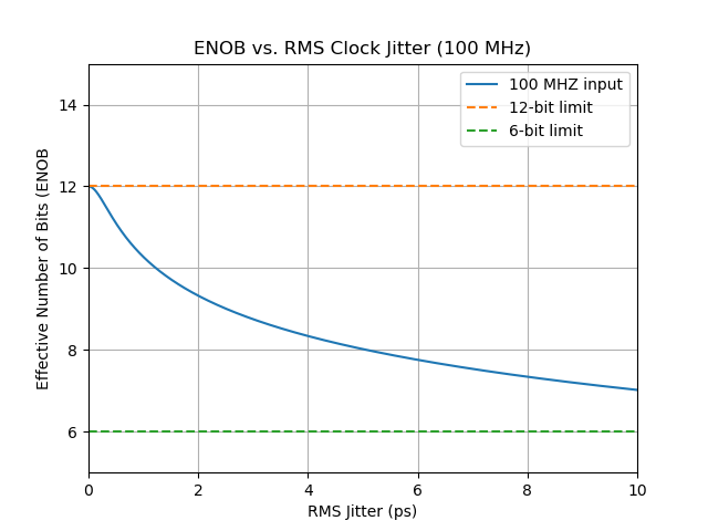
1 | import numpy as np |
Chun-Hsien Su (蘇純賢). Design of Oversampled Sigma-Delta Data Converters. July, 2006 [pdf]
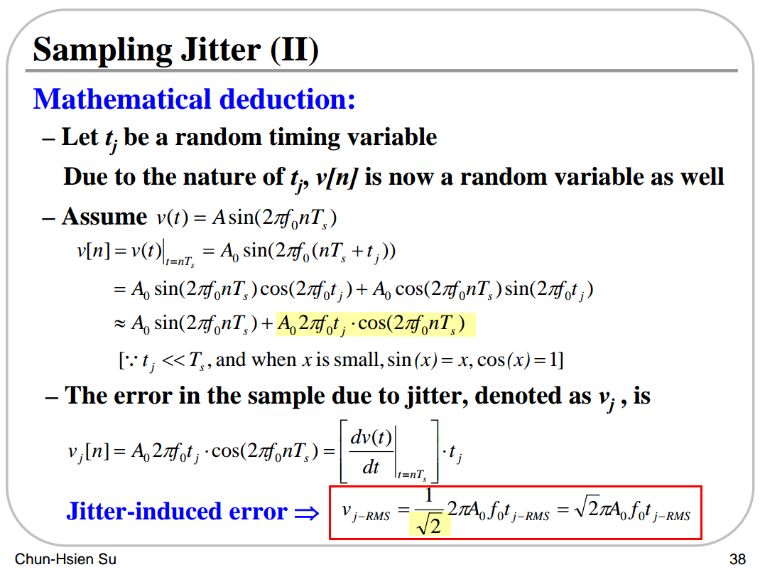
Chembian Thambidurai, "SNR of an ADC in the presence of clock jitter" [https://www.linkedin.com/posts/chembiyan-t-0b34b910_adcsnrjitter-activity-7171178121021304833-f2Wd/]
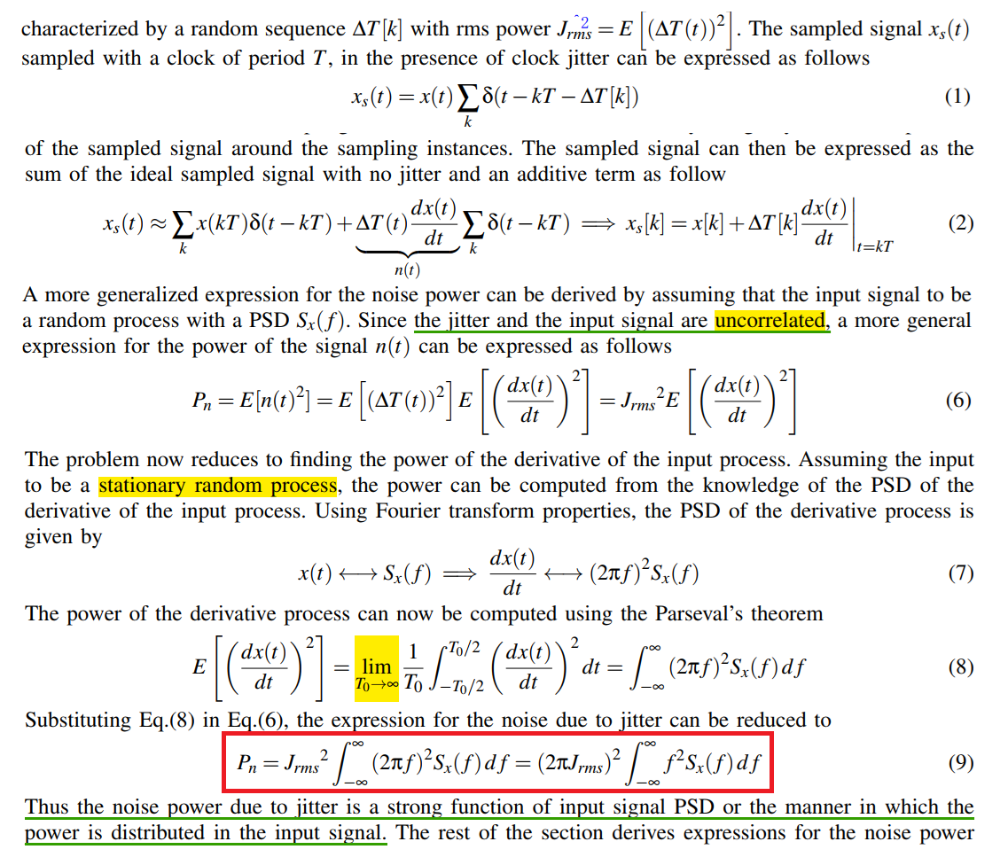
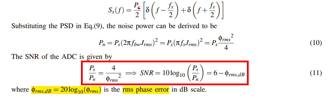
Unlike the quantization noise and the thermal noise, the impact of the clock jitter on the ADC performance depends on the input signal properties like its PSD
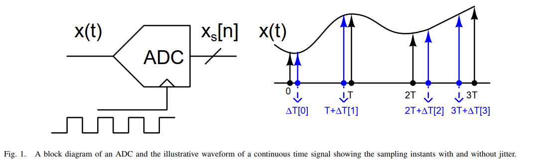
The error between the ideal sampled signal and the sampling with clock jitter can be treated as noise and it results in the degradation of the SNR of the ADC
For sinusoid input:
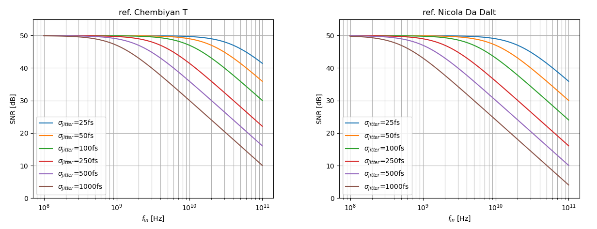
1 | import numpy as np |
K. Tyagi and B. Razavi, "Performance Bounds of ADC-Based Receivers Due to Clock Jitter," in IEEE Transactions on Circuits and Systems II: Express Briefs, vol. 70, no. 5, pp. 1749-1753, May 2023 [https://www.seas.ucla.edu/brweb/papers/Journals/KT_TCAS_2023.pdf]
N. Da Dalt, M. Harteneck, C. Sandner and A. Wiesbauer, "On the jitter requirements of the sampling clock for analog-to-digital converters," in IEEE Transactions on Circuits and Systems I: Fundamental Theory and Applications, vol. 49, no. 9, pp. 1354-1360, Sept. 2002 [https://sci-hub.se/10.1109/TCSI.2002.802353]
M. Shinagawa, Y. Akazawa and T. Wakimoto, "Jitter analysis of high-speed sampling systems," in IEEE Journal of Solid-State Circuits, vol. 25, no. 1, pp. 220-224, Feb. 1990 [https://sci-hub.se/10.1109/4.50307]
Akkaya, A. (2021). High-Speed ADC Design and Optimization for Wireline Links (Publication No. 8453) [PhD thesis, EPFL; Supervised by Y. Leblebici]. [https://doi.org/10.5075/epfl-thesis-8453]

待学芯. ADC量化结果反推采样时钟抖动(Jitter) [https://mp.weixin.qq.com/s/55xfVQMe_N8zUGpI8ZvmsQ]
—. 关于时钟抖动(Jitter)与ADC的一些讨论 [https://mp.weixin.qq.com/s/GW1keHhfq7zrd036lyG0CQ]
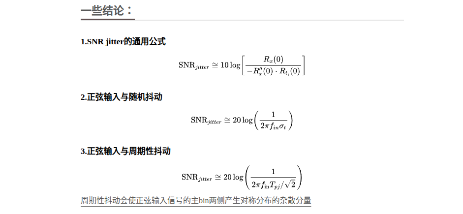
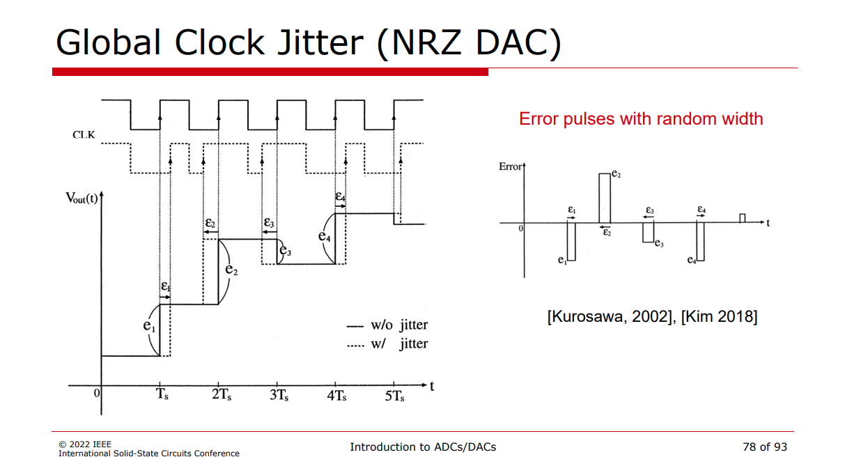
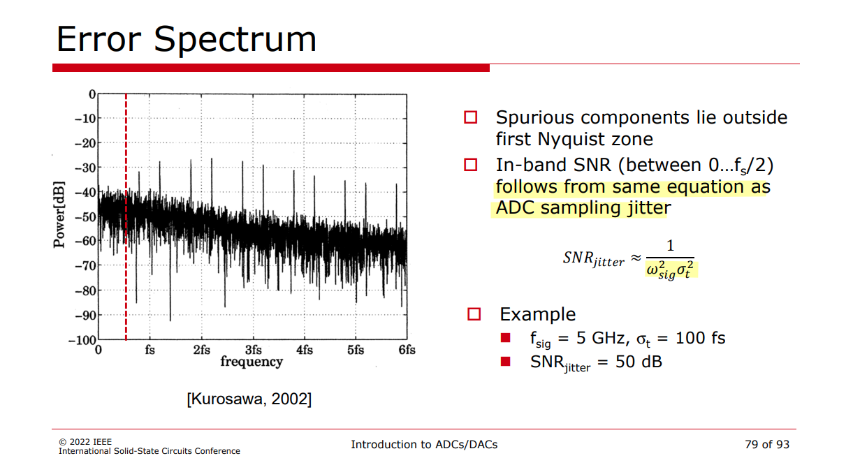
DAC SNR & clock jitter
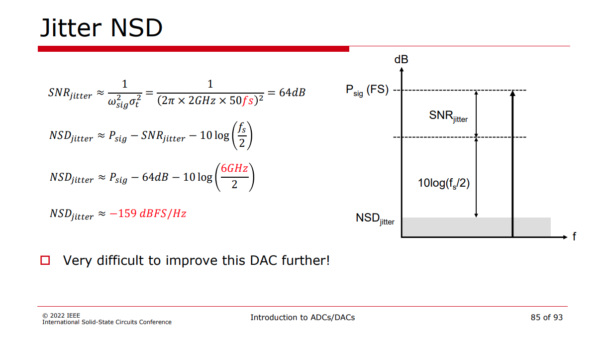
Boris Murmann ISSCC 2022 SC1: Introduction to ADCs/DACs: Metrics, Topologies, Trade Space, and Applications [pdf]
S. Kim, K. -Y. Lee and M. Lee, "Modeling Random Clock Jitter Effect of High-Speed Current-Steering NRZ and RZ DAC," in IEEE Transactions on Circuits and Systems I: Regular Papers, vol. 65, no. 9, pp. 2832-2841, Sept. 2018 [https://sci-hub.se/10.1109/TCSI.2018.2821198]
Martin Clara. High-Performance D/A-Converters - Application to Digital Transceivers, 2013 [pdf]
Chun-Hsien Su (蘇純賢). Design of Oversampled Sigma-Delta Data Converters. July, 2006 [pdf]
ampling Jitter Effects for ADC/DAC
- In both DAC or ADC cases, doubling the timing jitter doubles the noise level
- Also, doubling the frequency or amplitude doubles the jitter induced noise - SNR is not improved
ADC Linearity (DNL/INL)
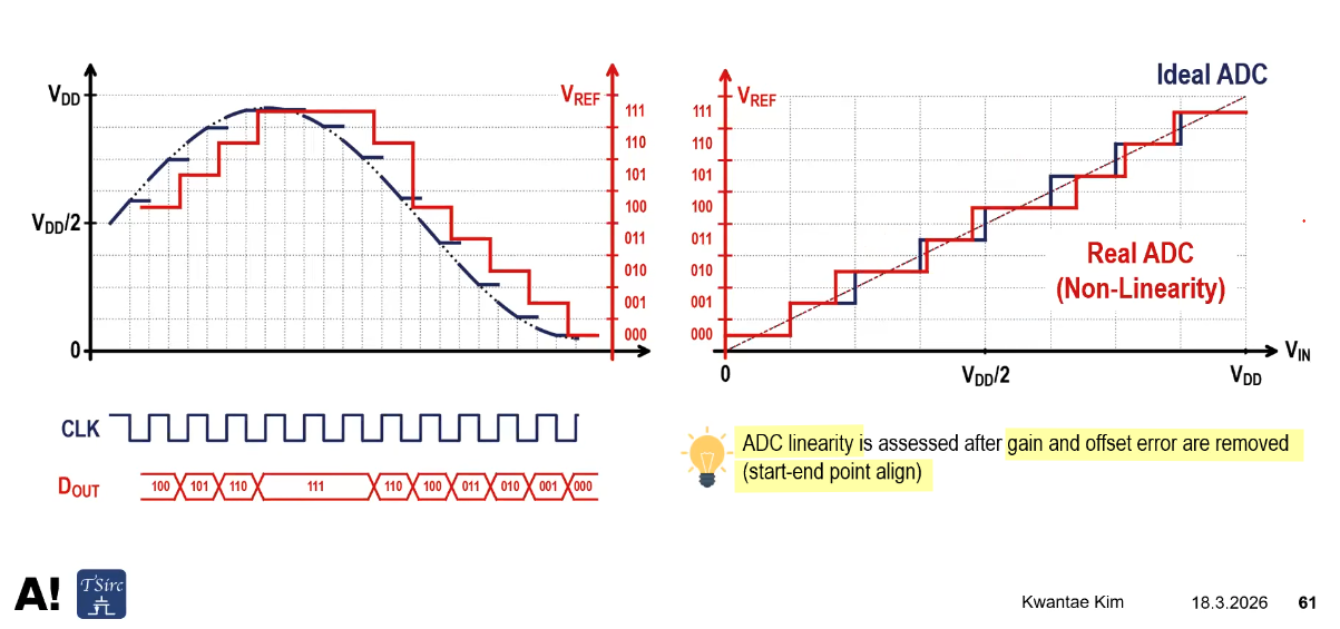
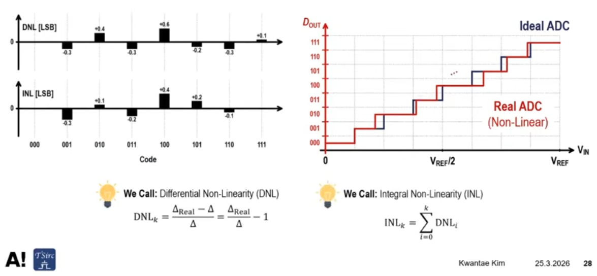
missing code
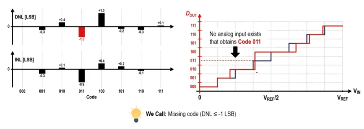
TODO 📅
EndpointmethodBestFitmethod
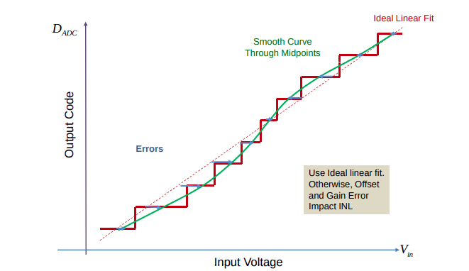
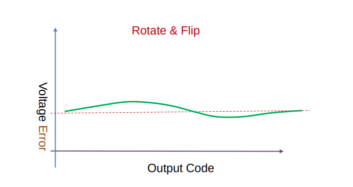
INL/DNL Measurements for High-Speed Analog-to Digital Converters (ADCs) [https://picture.iczhiku.com/resource/eetop/sYKTSqLfukeHSmMB.pdf]
Code Density Test
Apply a linear ramp to ADC input
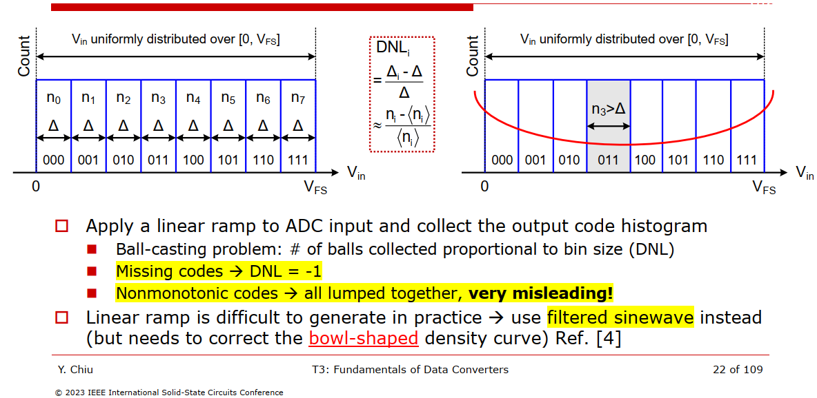
Jungwirth, Patrick. Sampling Theory and Analog-to-Digital Conversion. Independently published, 2018.
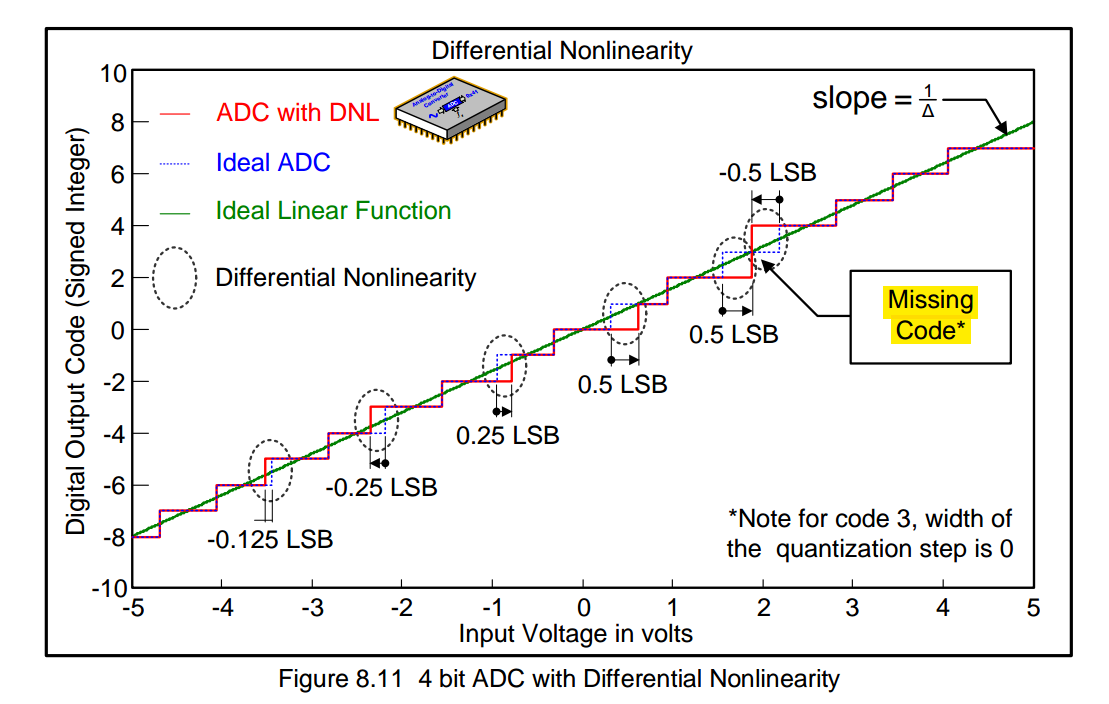
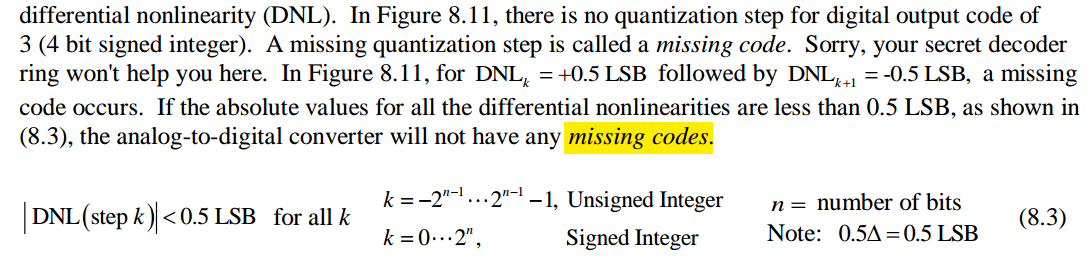
DAC Linearity (DNL/INL)
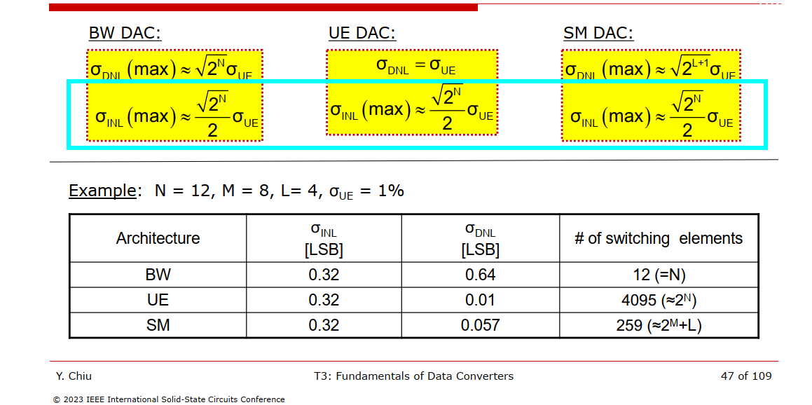
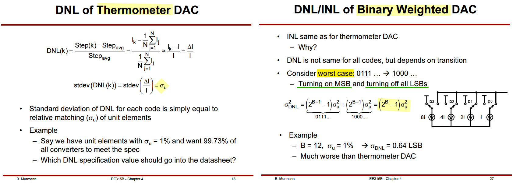
The worst INL of three DAC Architecture is same
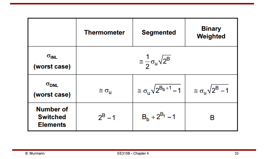
DAC DNL
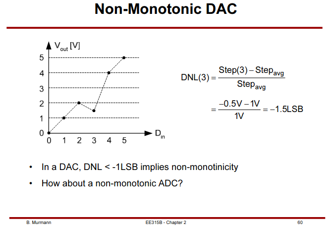
One difference between ADC and DAC is that DAC DNL can be less than -1 LSB
In a DAC, DNL < -1LSB implies non-monotonicity
DAC INL
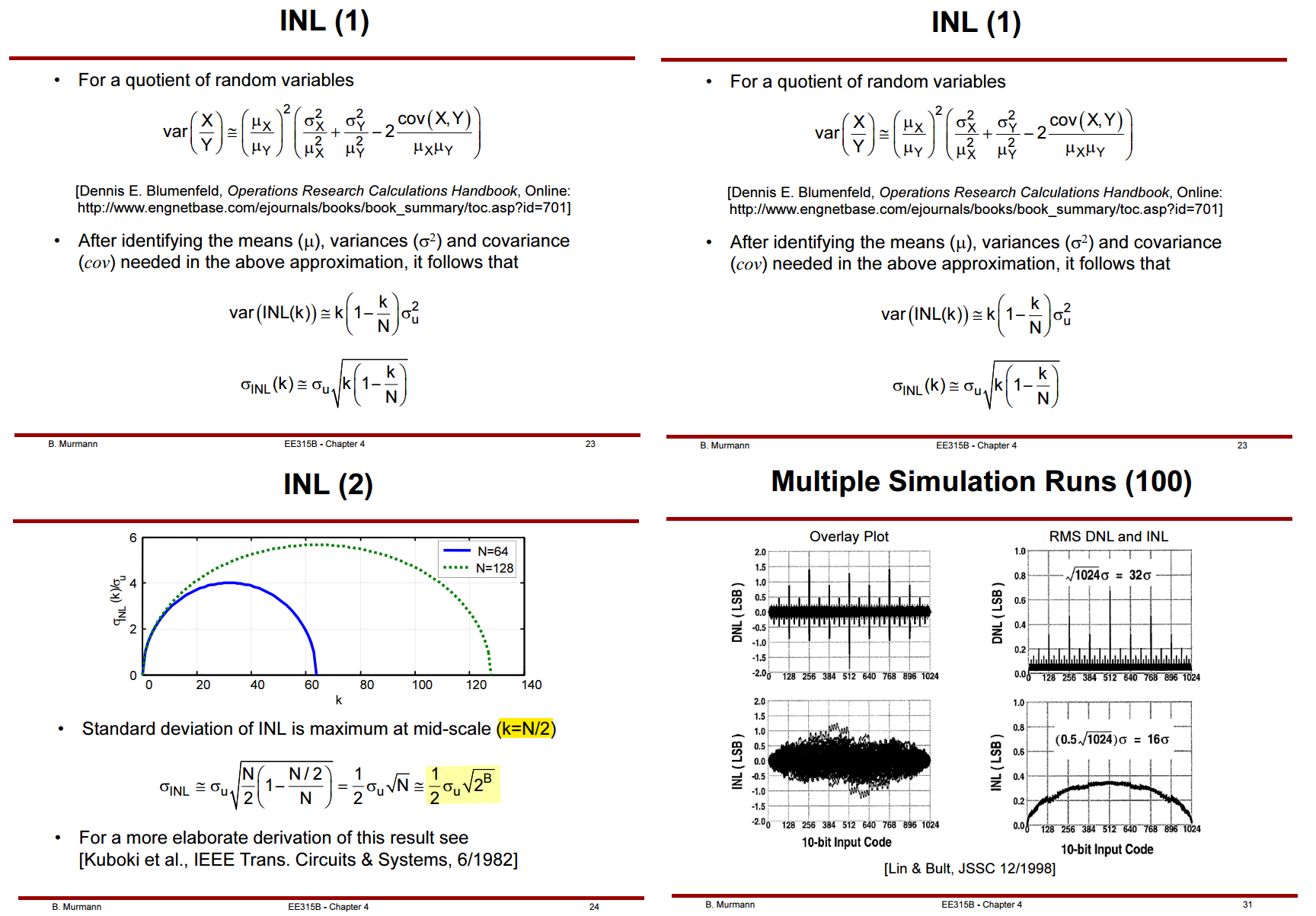
- \(A = \sum_{j=1}^k I_j\), \(B=\sum_{j=k+1}^N I_j\)
- A and B are independent with \(\sigma_A^2 = k\sigma_u^2\) and \(\sigma_B^2=(N-k)\sigma_u^2\)
Therefore \[ \mathrm{Var}\left(\frac{X}{Y}\right)\approx \frac{k^2}{N^2}\left(\frac{\sigma_i^2}{kI_u^2} + \frac{\sigma_i^2}{NI_u^2} -2\frac{\mathrm{cov}(X,Y)}{kNI_u^2}\right) \] and \[\begin{align} \mathrm{cov}(X,Y) &= E[XY] - E[X]E[Y] = E[A(A+B)] - kNI_u^2 \\ &= E[A^2]+E[A]E[B] - kNI_u^2= \sigma_A^2+E[A]^2 + k(N-k)I_u^2 - kNI_u^2\\ &= k\sigma_i^2 + k^2I_u^2+ k(N-k)I_u^2 - kNI_u^2 \\ &= k\sigma_i^2 \end{align}\]
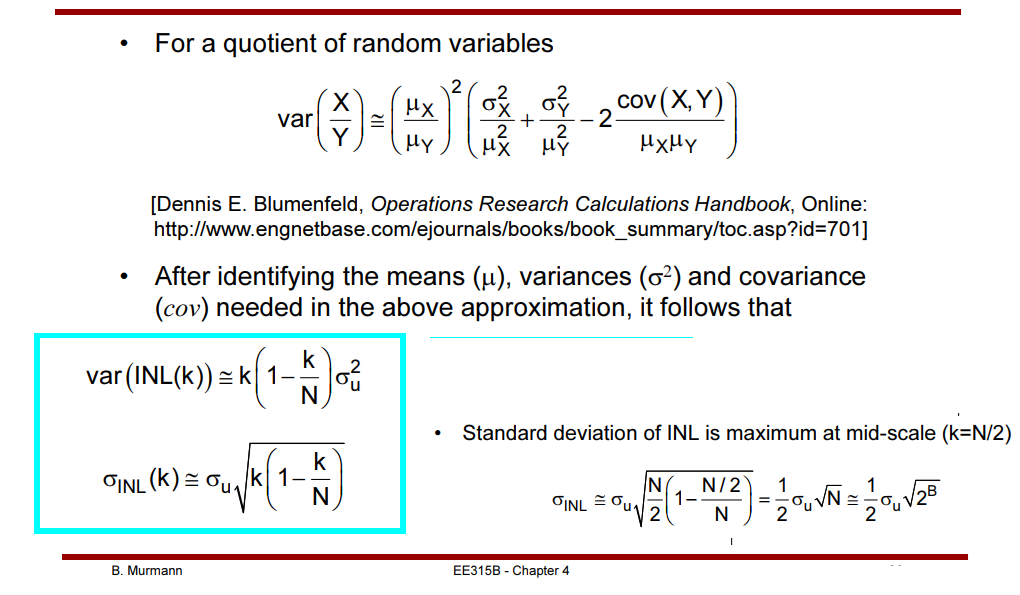
Finally, \[ \mathrm{Var}\left(\frac{X}{Y}\right)\approx \frac{k^2}{N^2}\left(\frac{\sigma_i^2}{kI_u^2} + \frac{\sigma_i^2}{NI_u^2} -2\frac{k\sigma_i^2}{kNI_u^2}\right) = \frac{k^2}{N^2}\left(\frac{1}{k}- \frac{1}{N}\right)\sigma_u^2 \] i.e. \[ \boxed{\mathrm{Var(INL(k))} = k^2\left(\frac{1}{k}- \frac{1}{N}\right)\sigma_u^2 = k\left(1- \frac{k}{N}\right)\sigma_u^2} \]
Standard deviation of INL is maximum at mid-scale (k=N/2)
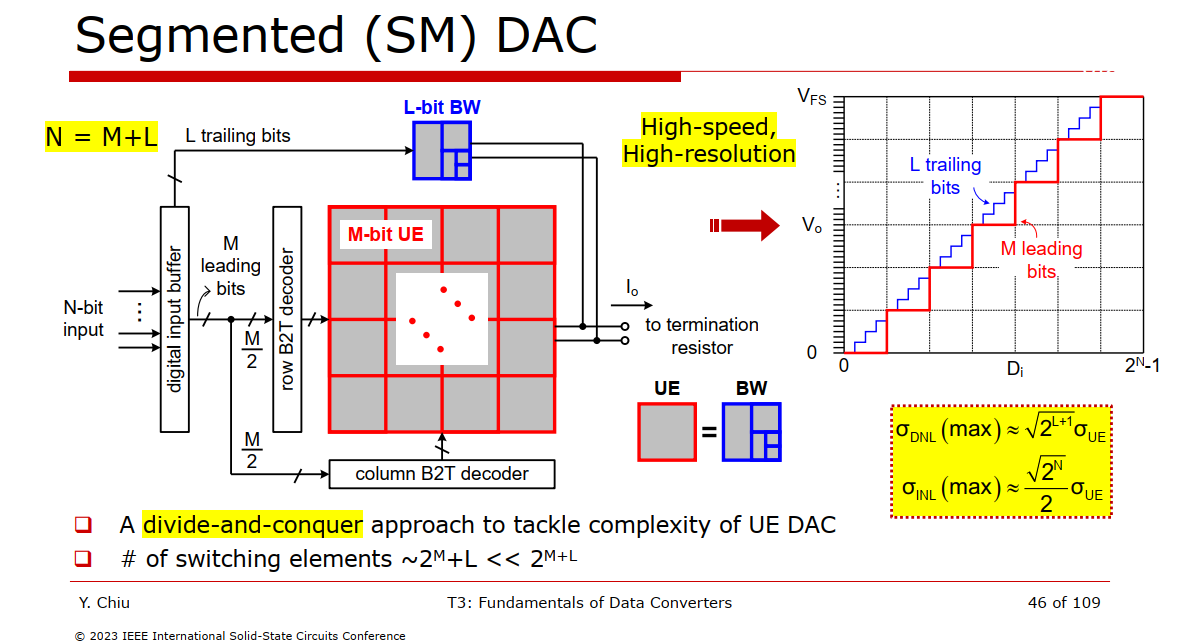
INL/DNL analysis of current steering DAC
Spectral Metrics
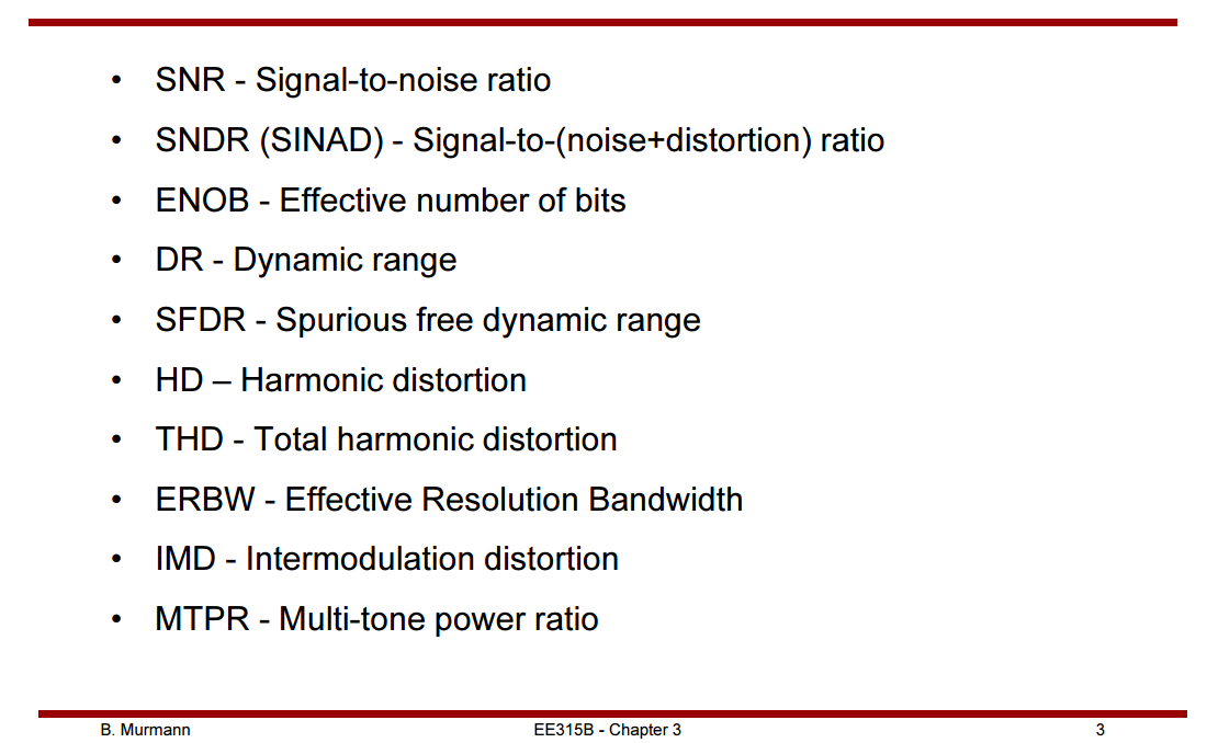
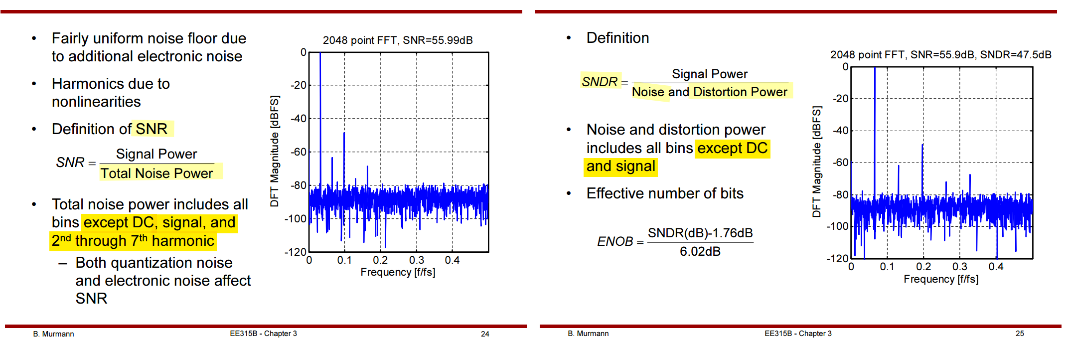
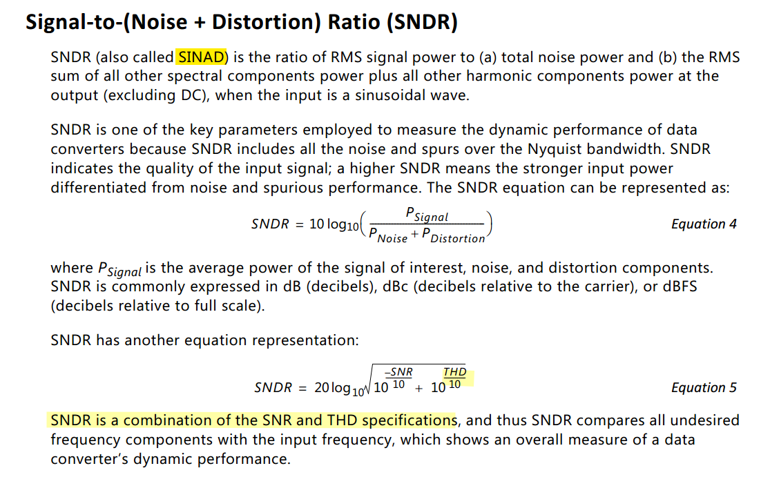
SNR, SNDR (SINAD)
Understanding Key Parameters for RF-Sampling Data Converters White Paper (WP509) [https://docs.amd.com/v/u/en-US/wp509-rfsampling-data-converters]
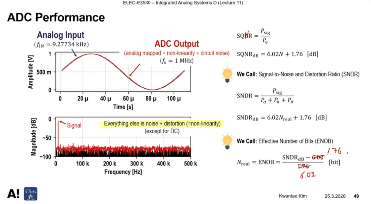
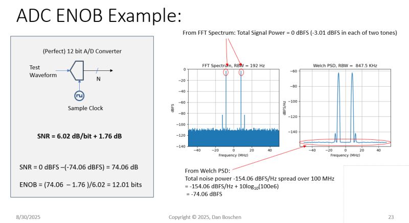
ENOB
Qasim Chaudhari, On Analog-to-Digital Converter (ADC), 6 dB SNR Gain per Bit, Oversampling and Undersampling [https://wirelesspi.com/on-analog-to-digital-converter-adc-6-db-snr-gain-per-bit-oversampling-and-undersampling/]
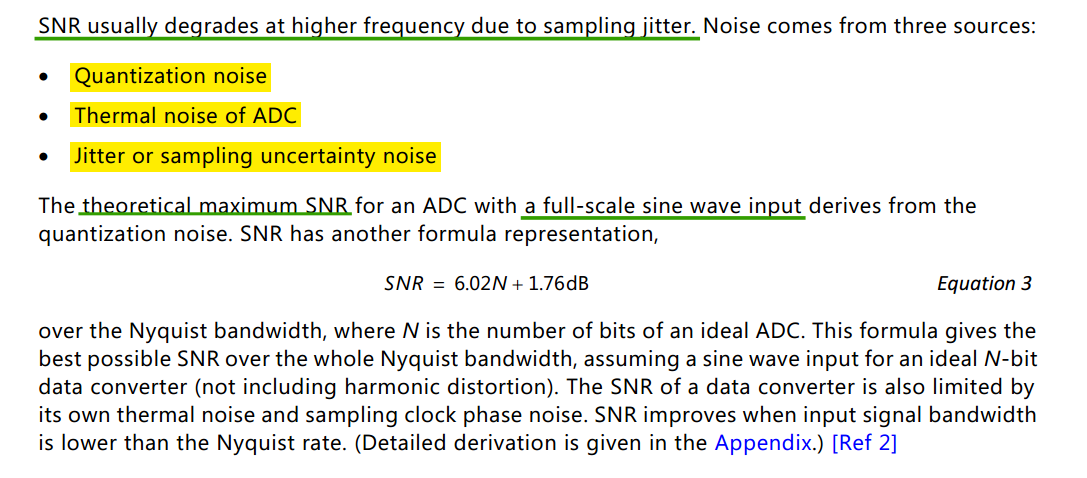
The quantization noise power \(P_Q\) for a uniform quantizer with step size \(\Delta\) is given by \[ P_Q = \frac{\Delta ^2}{12} \] For a full-scale sinusoidal input signal with an amplitude equal to \(V_{FS}/2\), the input signal is given by \(x(t) = \frac{V_{FS}}{2}\sin(\omega t)\)
Then input signal power \(P_s\) is \[ P_s = \frac{V_{FS}^2}{8} \] Therefore, the signal-to-quantization noise ratio (SQNR) is given by \[ \text{SQNR} = \frac{P_s}{P_Q} = \frac{V_{FS}^2/8}{\Delta^2/12}=\frac{V_{FS}^2/8}{V_{FS}^2/(12\times 2^{2N})} = \frac{3\times 2^{2N}}{2} \] where \(N\) is the number of quantization bits
When represented in dBs \[ \text{SQNR(dB)} = 10\log(\frac{P_s}{P_Q}) = 10\log(\frac{3\times 2^{2N}}{2})= 20N\log(2) + 10\log(\frac{3}{2})= 6.02N + 1.76 \]
the maximum achievable SNR of N-bit ADC — theoretical SNR limit
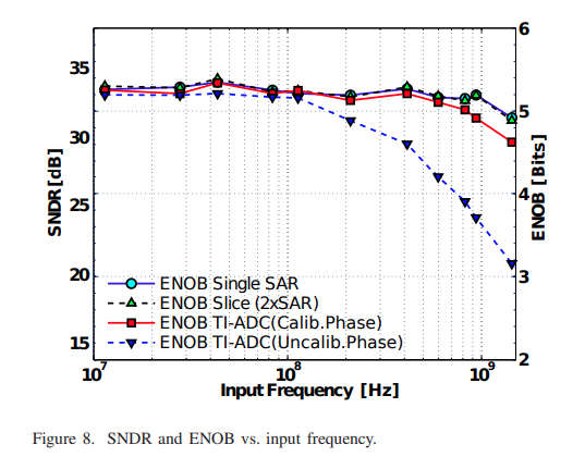
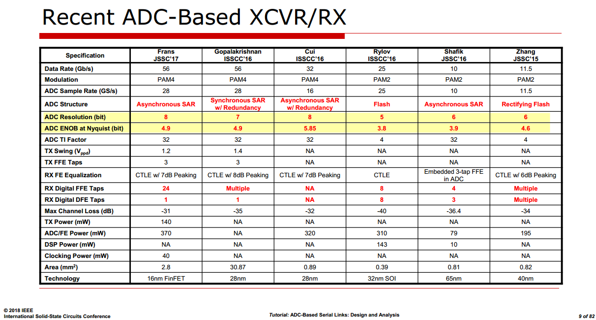
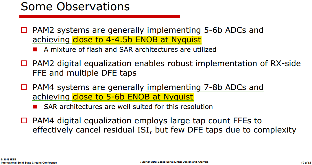
Dan Boschen, GRCon25: Quantifying Signal Quality: Practical Tools for High-Fidelity Waveform Analysis
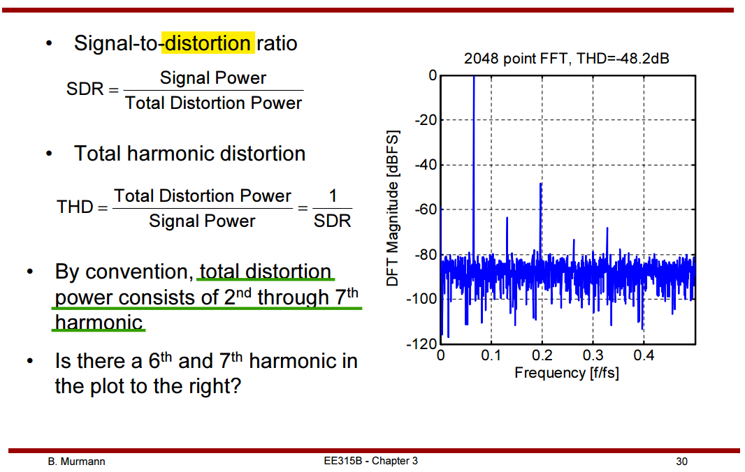
SDR, THD
Understanding Key Parameters for RF-Sampling Data Converters White Paper (WP509) [https://docs.amd.com/v/u/en-US/wp509-rfsampling-data-converters]
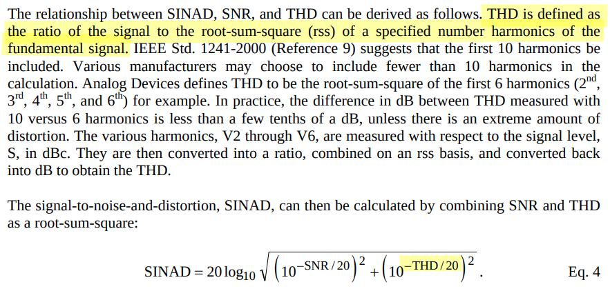
Walt Kester. Evaluating High Speed DAC Performance [https://www.analog.com/media/en/training-seminars/tutorials/mt-013.pdf]
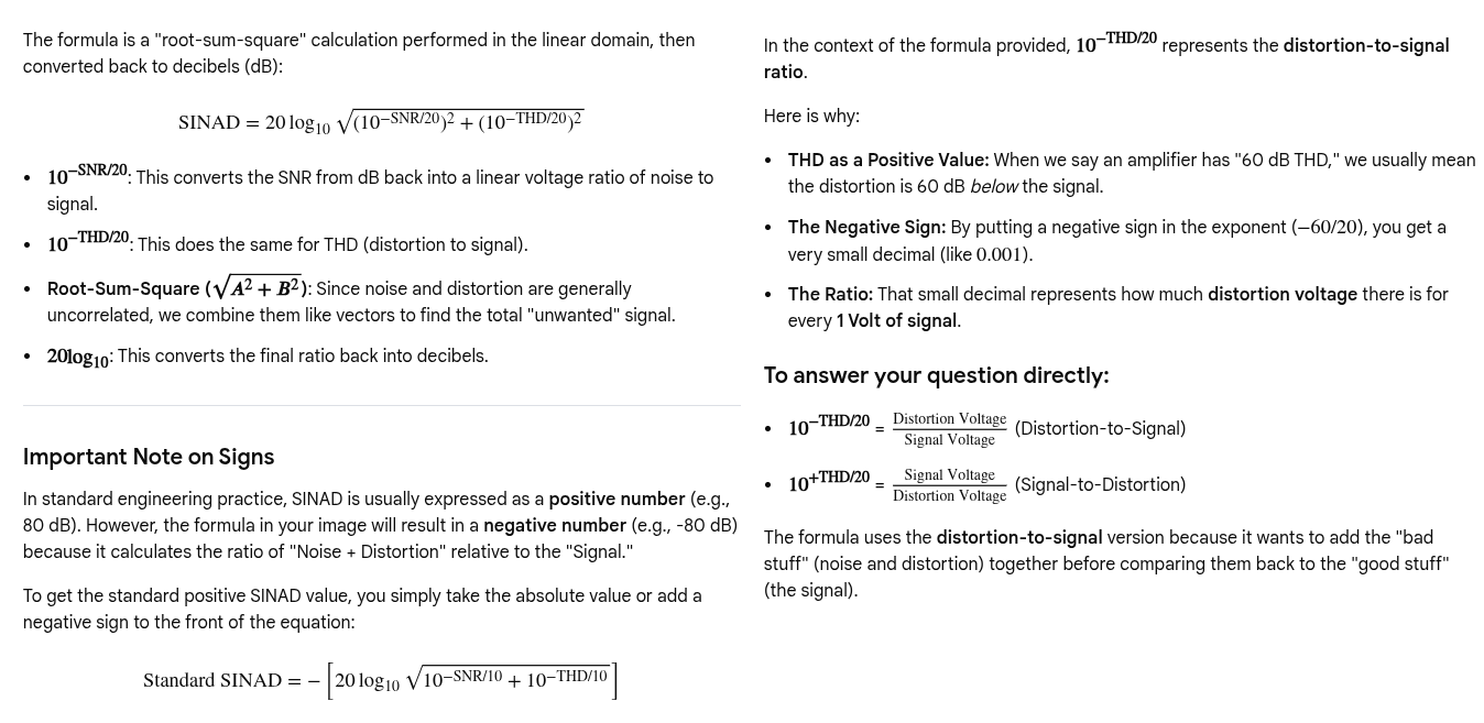
via other definition
THD: signal to distortion
SINAD: noise and distortion to signal
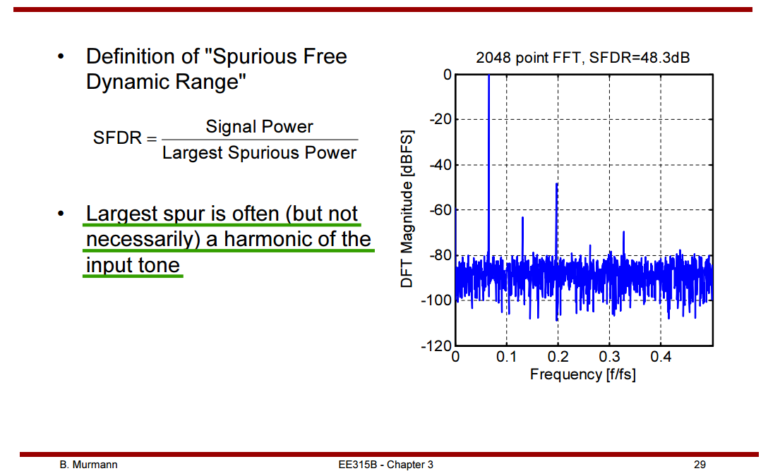
SFDR & INL
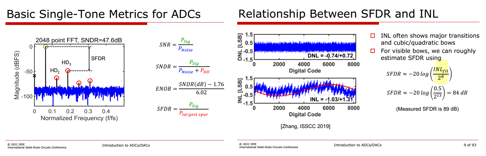
Beware, this is of course only true under the same conditions at which the INL was taken, i.e. typically low input signal frequency
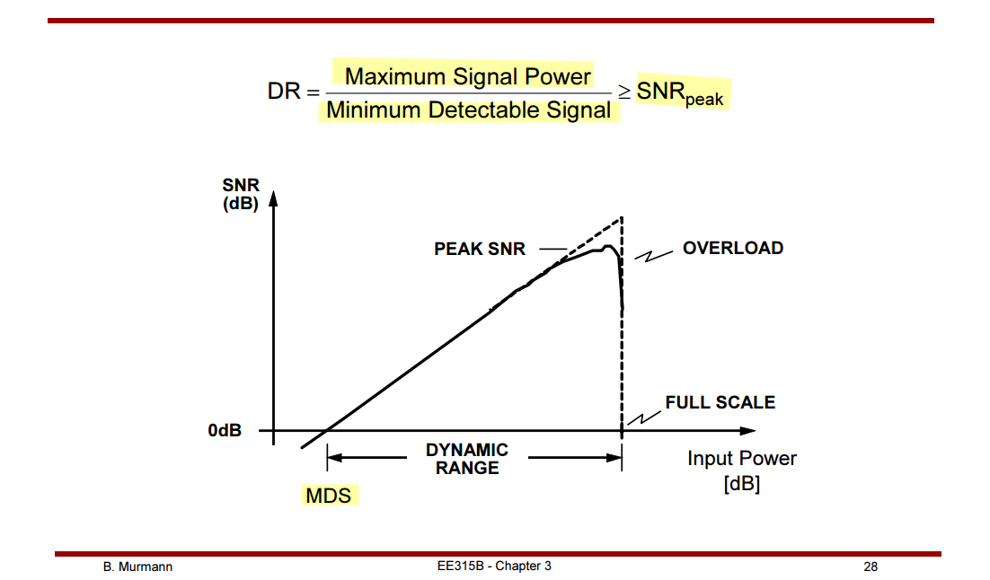
Dynamic Range (DR)
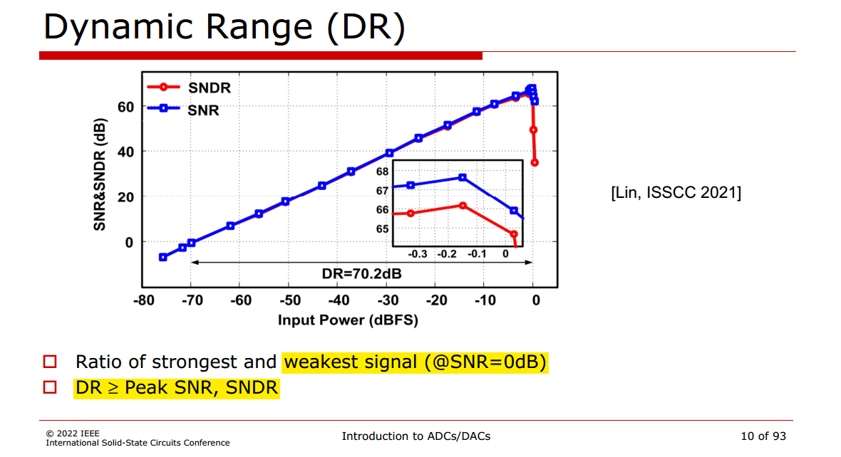
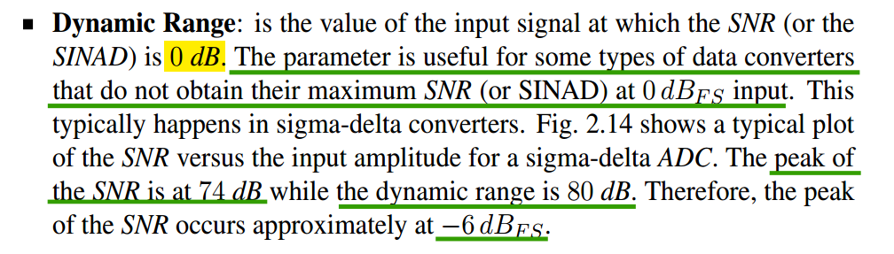
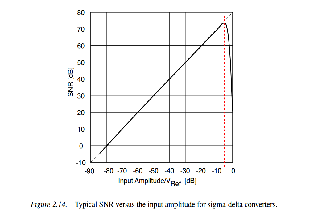
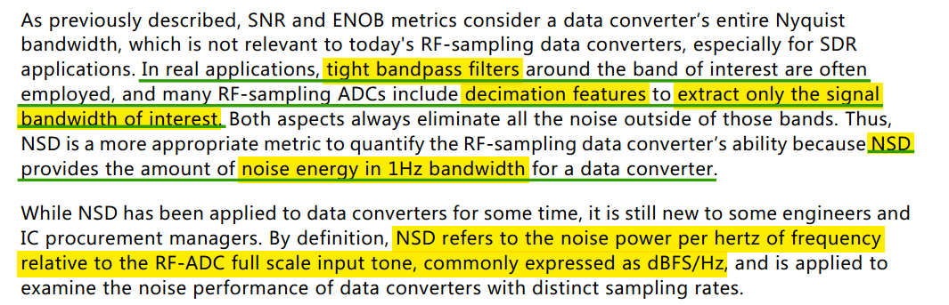
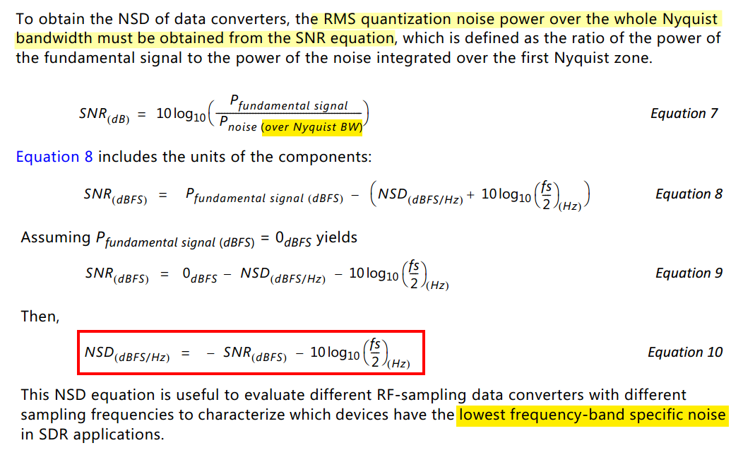
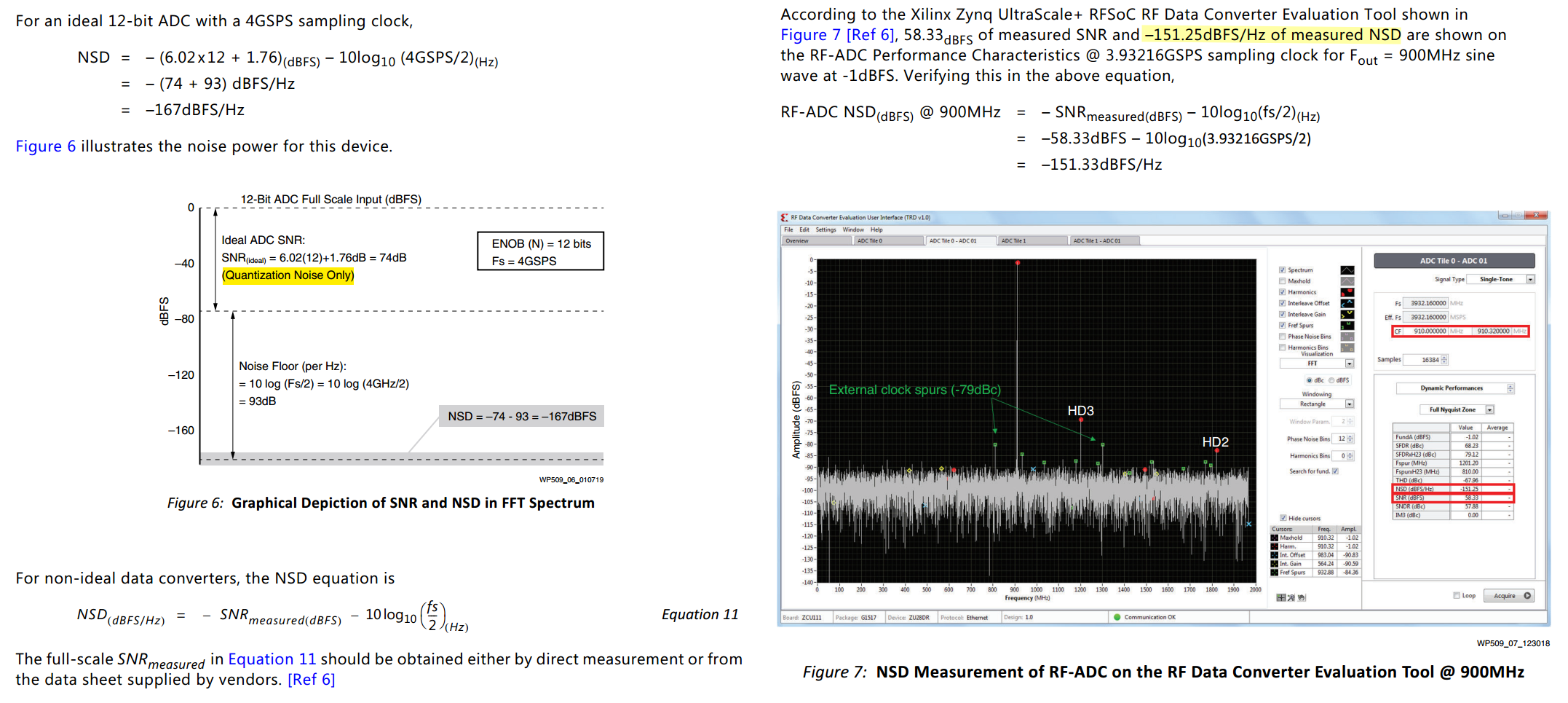
Noise Spectral Density (NSD)
Understanding Key Parameters for RF-Sampling Data Converters White Paper (WP509) [https://docs.amd.com/v/u/en-US/wp509-rfsampling-data-converters]
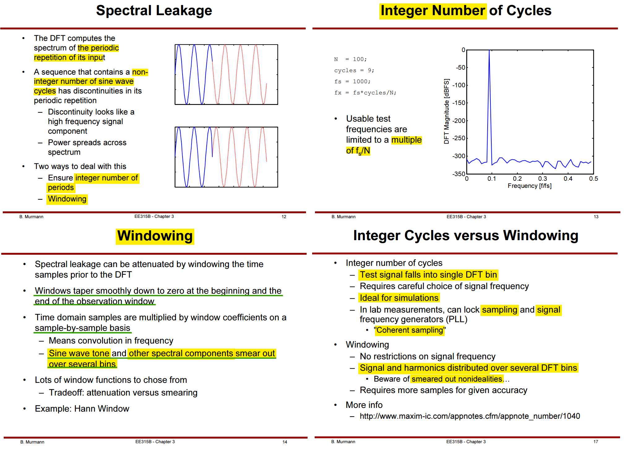
Spectral Leakage
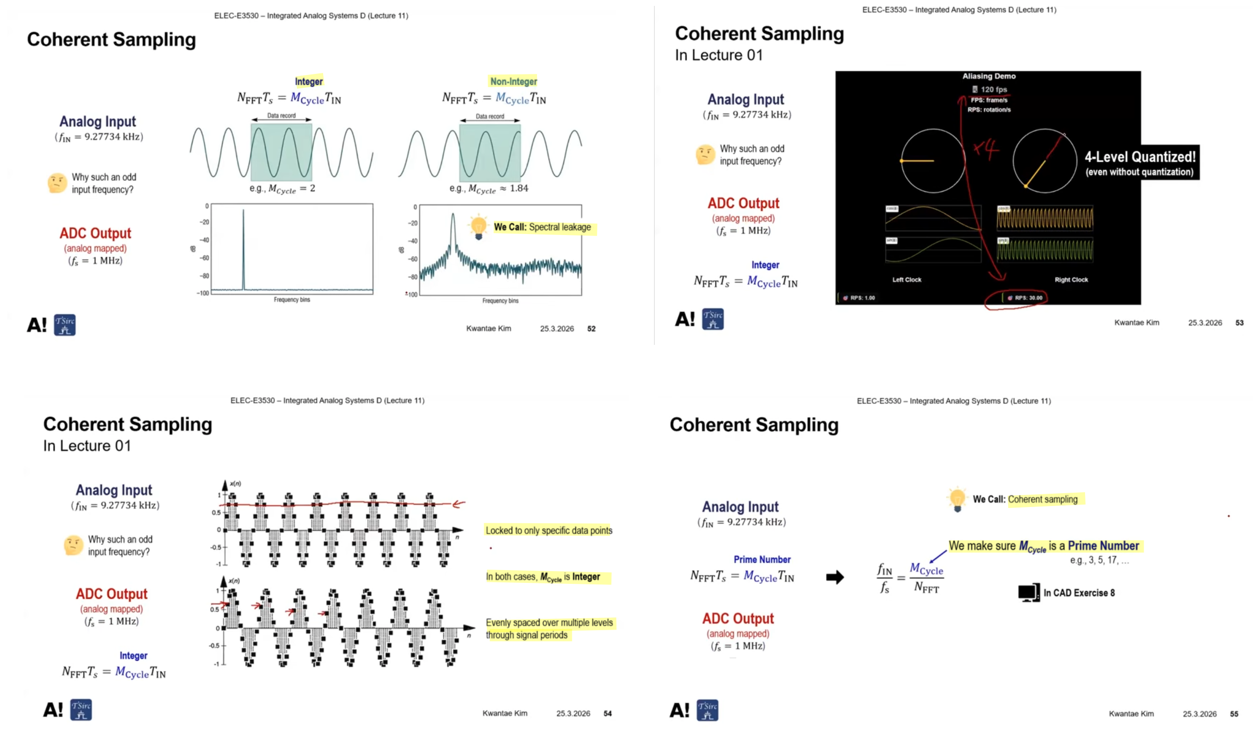
Two ways to deal with spectral leakage: Ensure integer number of periods or Windowing
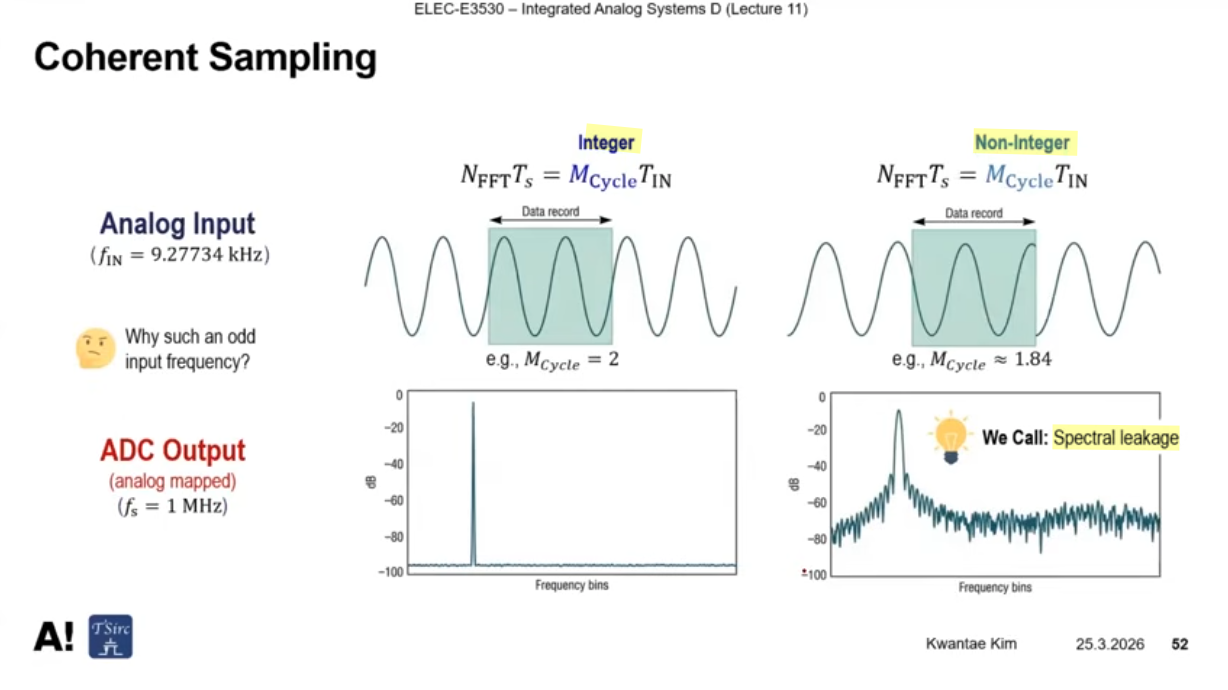
Coherent Sampling
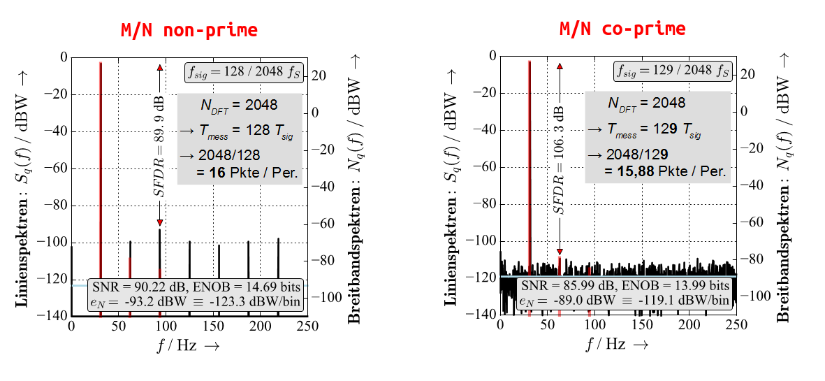
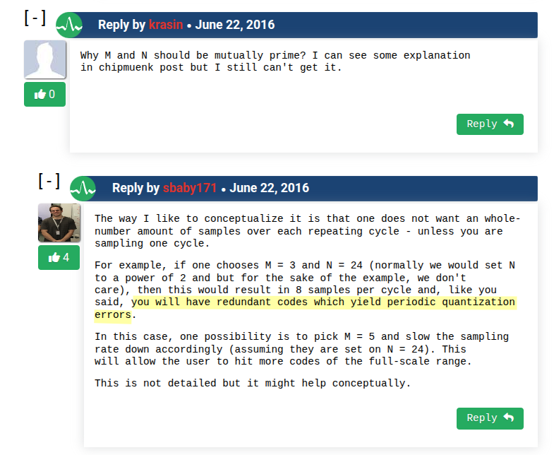
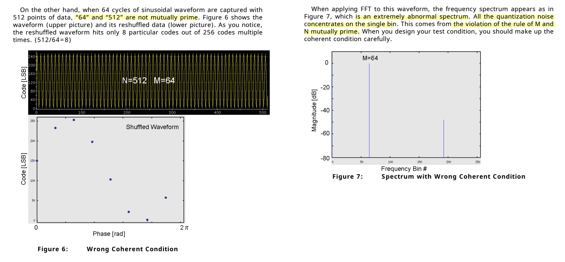
Choosing M/N non-prime repeats the signal quantization periodically and fewer quantization steps are measured. The quantization repeats periodically and creates a line spectrum that can obscure real frequency lines (e.g. the red lines in the images below, created by non-linearities of the ADC).[https://www.dsprelated.com/thread/469/coherent-sampling-very-brief-and-simple]
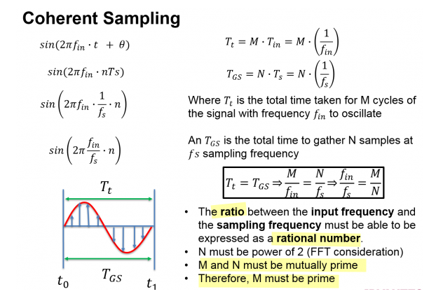
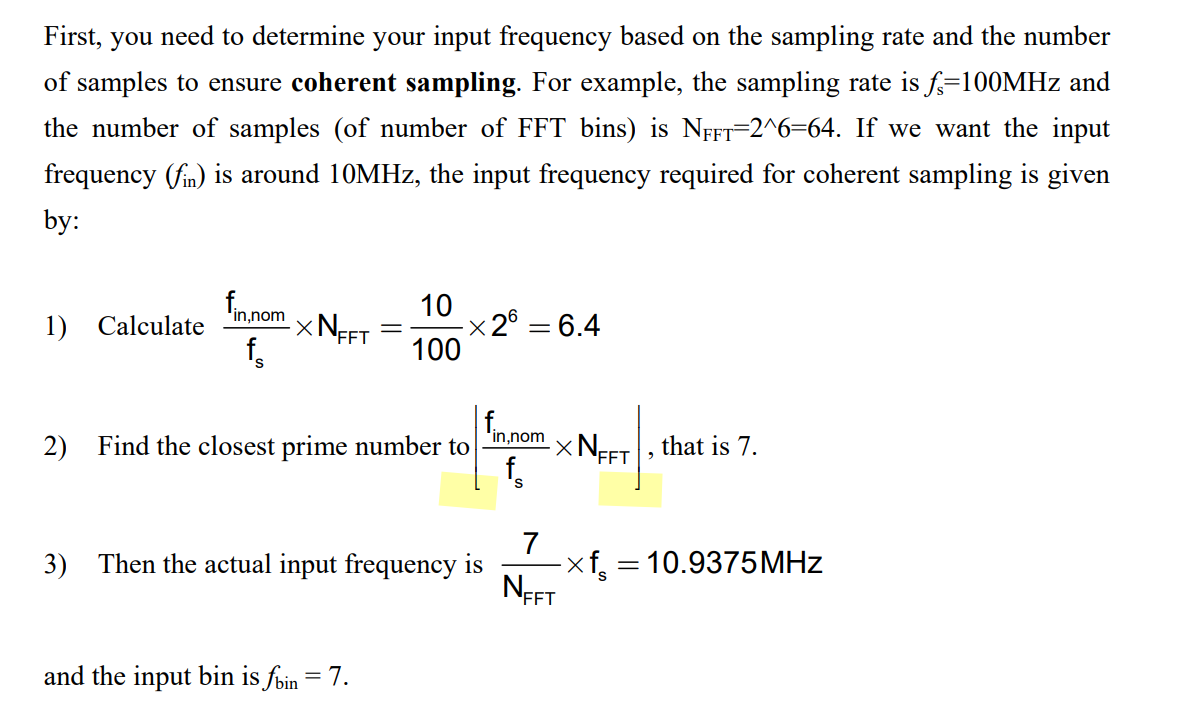
\[ \frac{f_{\text{in}}}{f_{\text{s}}}=\frac{M_C}{N_R} \]
\(f_\text{in}\) and \(f_s\) must be incommensurate (\(f_s/f_\text{in}\) is irrational number. btw, co-prime is sufficient but not necessary)
\(M_C\) and \(N_R\) must be co-prime
Samples must include integer # of cycles of input signal
An irreducible ratio ensures identical code sequences not to be repeated multiple times.
Given that \(\frac{M_C}{N_R}\) is irreducible, and \(N_R\) is a power of 2, an odd number for \(M_C\) will always produce an irreducible ratio
Assuming there is a common factor \(k\) between \(M_C\) and \(N_R\), i.e. \(\frac{M_C}{N_R}=\frac{k M_C'}{k N_R'}\)
The samples (\(n\in[1, N_R]\))
\[ y[n] = \sin\left( \omega_{\text{in}} \cdot t_n \right) = \sin\left( \omega_{\text{in}} \cdot n\frac{1}{f_s} \right) = \sin\left( \omega_{\text{in}} \cdot n\frac{1}{f_{\text{in}}}\frac{M_C}{N_R} \right) = \sin\left( 2\pi n\frac{M_C}{N_R} \right) \]
Then
\[ y[n+N_R'] = \sin\left( 2\pi (n+N_R')\frac{M_C}{N_R} \right) = \sin\left( 2\pi n \frac{M_C}{N_R} + 2\pi N_R'\frac{M_C}{N_R}\right) = \sin\left( 2\pi n \frac{M_C}{N_R} + 2\pi N_R'\frac{kM_C'}{kN_R'} \right) = \sin\left( 2\pi n \frac{M_C}{N_R}\right) \]
So, the samples is repeated \(\color{red}y[n] = y[n+N_R']\)
\(N_R\) & \(M_C\) irreducible ratio (mutually prime)
- Periodic sampling points result in periodic quantization errors
- Periodic quantization errors result in harmonic distortion
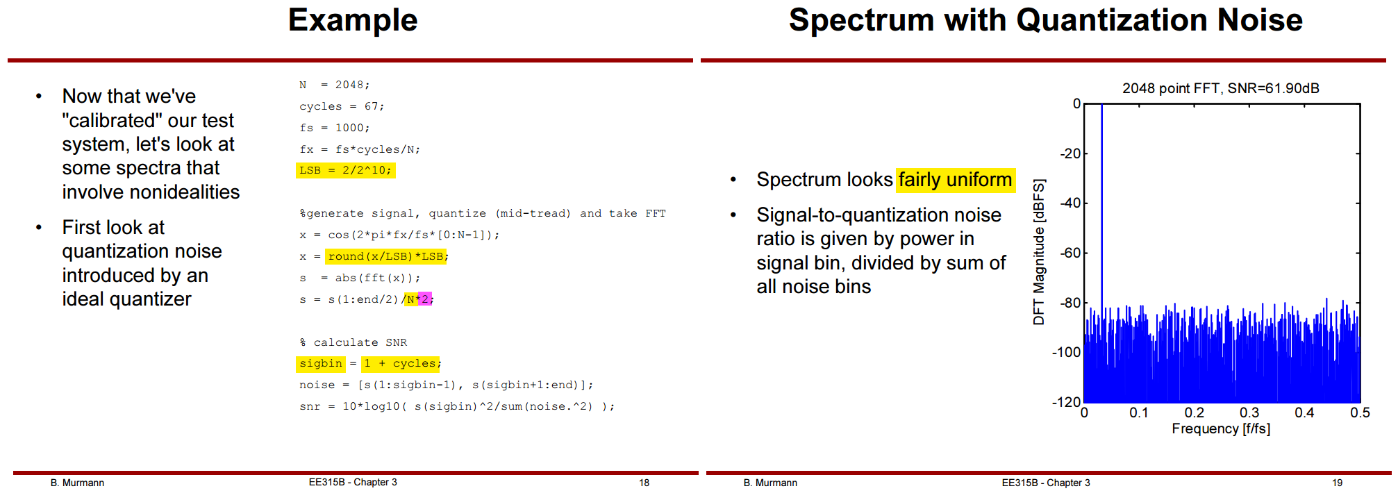
GCD(2048, 67)=1
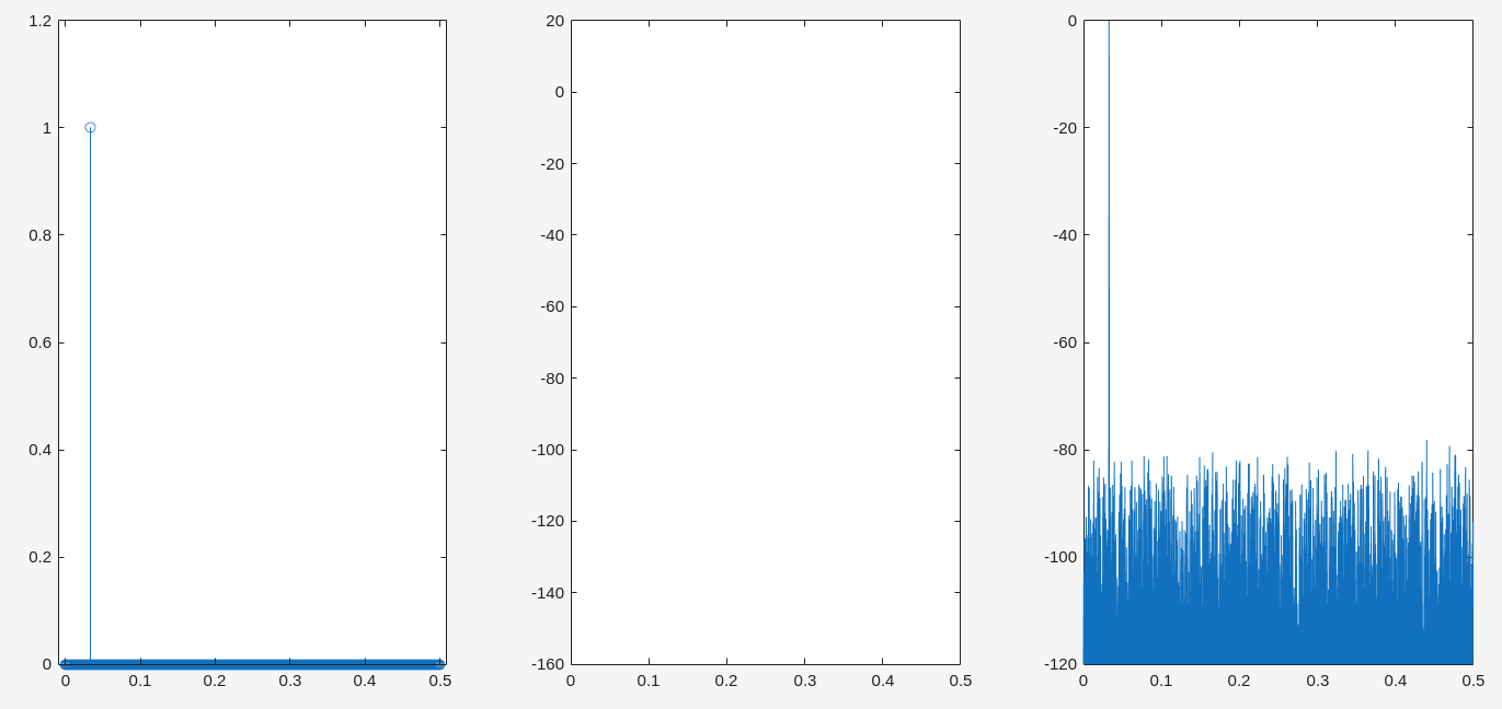
1 | N = 2048; |
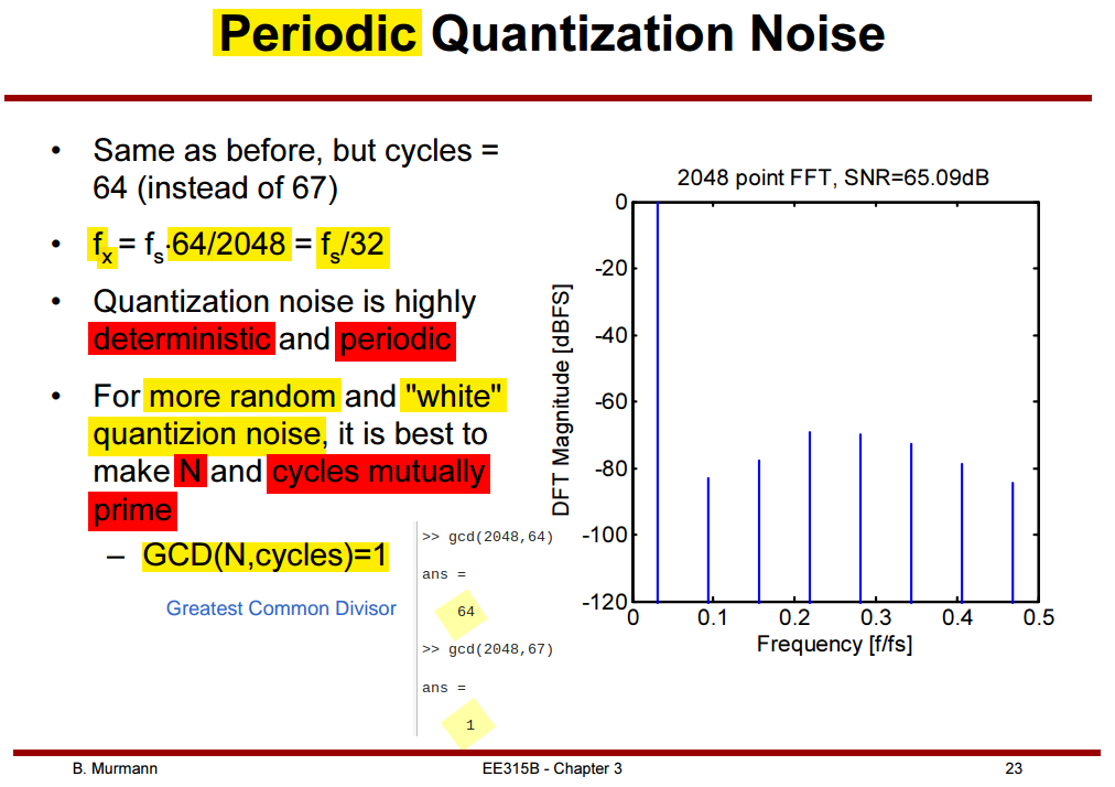
Periodic Quantization Noise if N and cycles
are not mutually prime, i.e.
cycles=64 then GCD(2048, 64)=64, then \(N_R' = 2048/64=32\), so quantization
noise manifests as odd harmonics \(n/32\mid n = 2k + 1, k \in \mathbb{Z}\)
because of Half Wave Symmetry
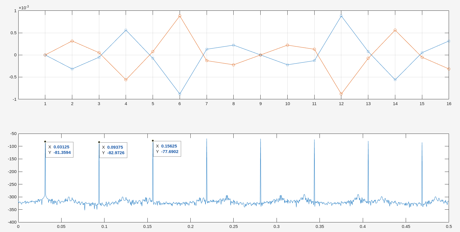
1 | N = 2048; |

Using FFT in Cadence Spectre [https://www.eecis.udel.edu/~vsaxena/courses/ece614/f14/Homeworks/fft_calculation.pdf]
Hideo Okawara's Mixed Signal Lecture Series, DSP-Based Testing - Fundamentals 6 - Spectrum Analysis – FFT [https://www3.advantest.com/documents/11348/8c5e06b8-85b8-407d-b253-b671ca9ac85c]
—, DSP-Based Testing - Fundamentals 7 - Coherent Condition [https://www3.advantest.com/documents/11348/7f5f00bb-f5f0-41da-b154-fc1d974ad201]
Kwantae Kim, ELEC-E3530 [https://github.com/KwantaeKim/ELEC-E3530/blob/main/CAD8.ipynb]
1 | import numpy as np |
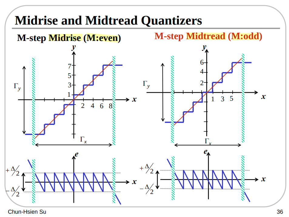
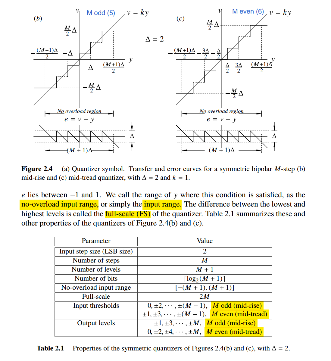
Midrise vs Midtread Quantizers
\(\Gamma_x\) is no-overload range
Top-Plate vs Bottom-Plate Sampling
[https://class.ece.iastate.edu/ee435/lectures/EE%20435%20Lect%2044%20Spring%202008.pdf]
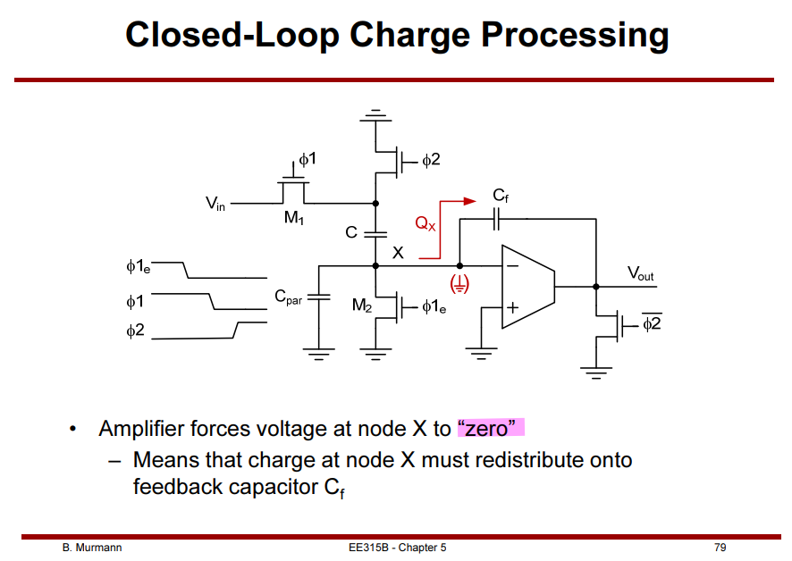
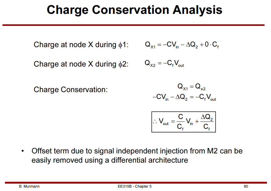
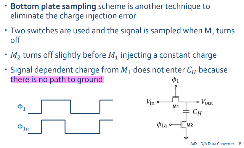
Bottom-Plate Sampling
Sample signal at the "grounded" side of the capacitor to achieve signal independent sampling
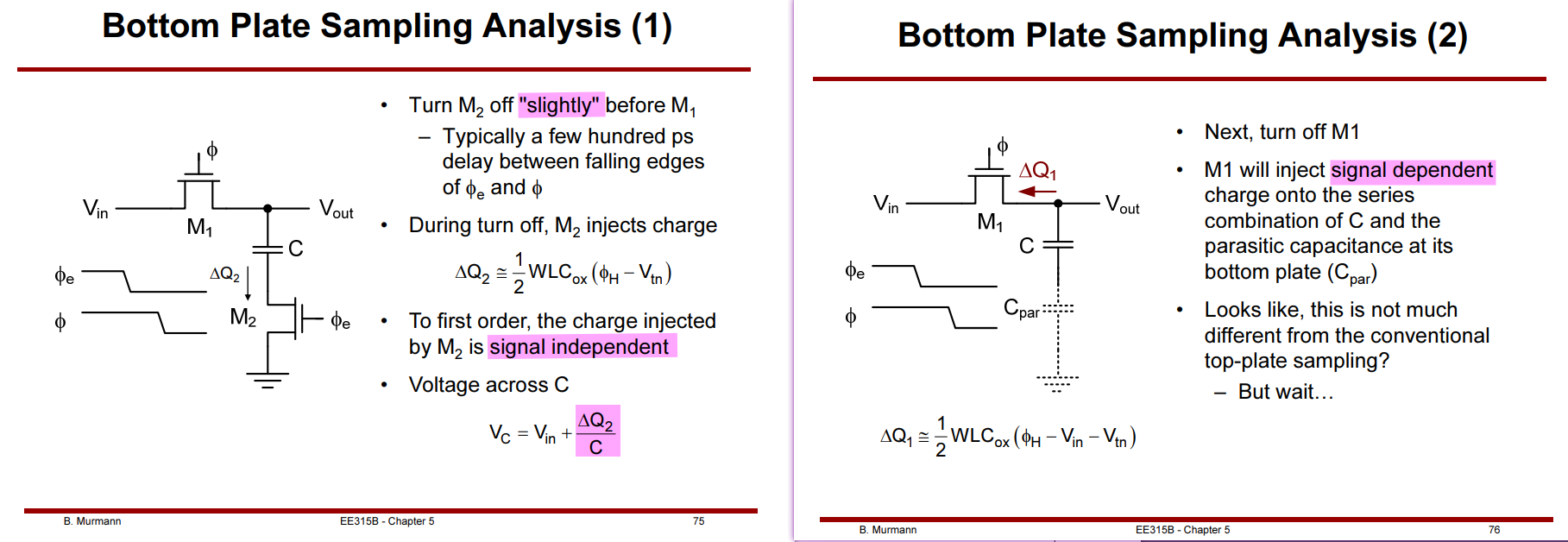
The capacitor voltage is defined as
\[ V_C = V_{\text{out}}-V_X \]
Before \(M_2\) turns off, \(M_1\) and \(M_2\) are both ON, so approximately
\[ V_{\text{out}}=V_{\text{in}},\qquad V_X=0 \]
and therefore
\[ V_C=V_{\text{in}} \]
When \(M_2\) turns off first, the slide writes
\[ V_C=V_{\text{in}}+\frac{\Delta Q_2}{C} \]
At this moment \(M_1\) is still ON, so the top plate is still held at
\[ V_{\text{out}}\approx V_{\text{in}} \]
Hence
\[\begin{aligned} V_X &=V_{\text{out}}-V_C\\ &=V_{\text{in}} -\left(V_{\text{in}}+\frac{\Delta Q_2}{C}\right)\\ &=\boxed{-\frac{\Delta Q_2}{C}}. \end{aligned}\]
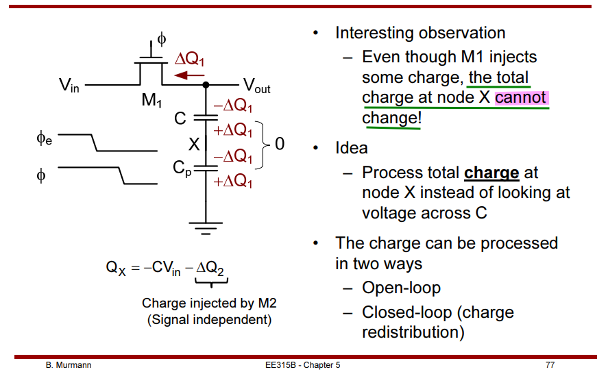
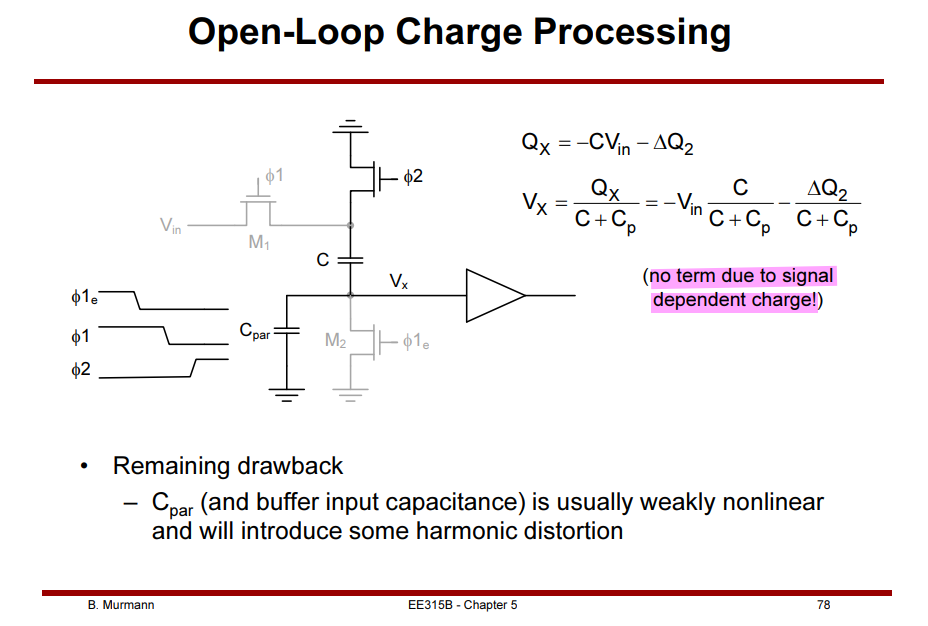
EE 435 Spring 2024 Analog VLSI Circuit Design - Switched-Capacitor Amplifiers Other Integrated Filters, https://class.ece.iastate.edu/ee435/lectures/EE%20435%20Lect%2044%20Spring%202008.pdf
Top-Plate Sampling
TODO 📅
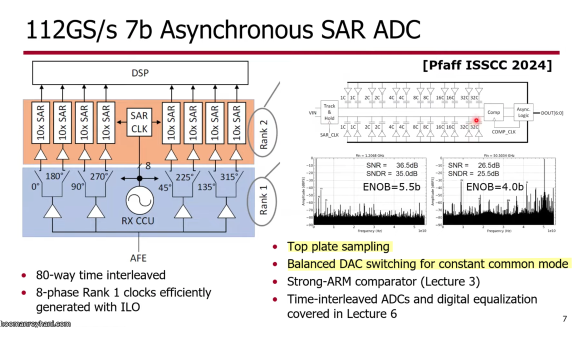
Maintain constant common-mode during conversion
D. Pfaff et al., "7.3 A 224Gb/s 3pJ/b 40dB Insertion Loss Transceiver in 3nm FinFET CMOS," 2024 IEEE International Solid-State Circuits Conference (ISSCC), San Francisco, CA, USA, 2024 [https://iccircle.com/static/upload/img20240529101747.pdf]
—, "A 224Gb/s 3pJ/bit 42dB Insertion Loss Post-FEC Error Free Transceiver in 3-nm FinFET CMOS (Invited)," 2025 IEEE Custom Integrated Circuits Conference (CICC), Boston, MA, USA, 2025, pp. 1-8, doi: 10.1109/CICC63670.2025.10983461.
E. Swindlehurst et al., "An 8-bit 10-GHz 21-mW Time-Interleaved SAR ADC With Grouped DAC Capacitors and Dual-Path Bootstrapped Switch," IEEE Journal of Solid-State Circuits, vol. 56, no. 8, pp. 2347-2359, 2021, [https://sci-hub.se/10.1109/JSSC.2021.3057372]
Tracking nonidealities
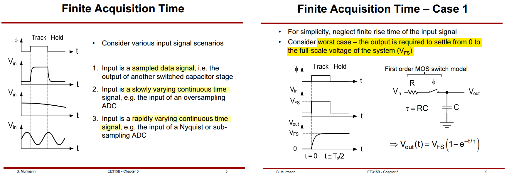
Tracking Settling Accuracy
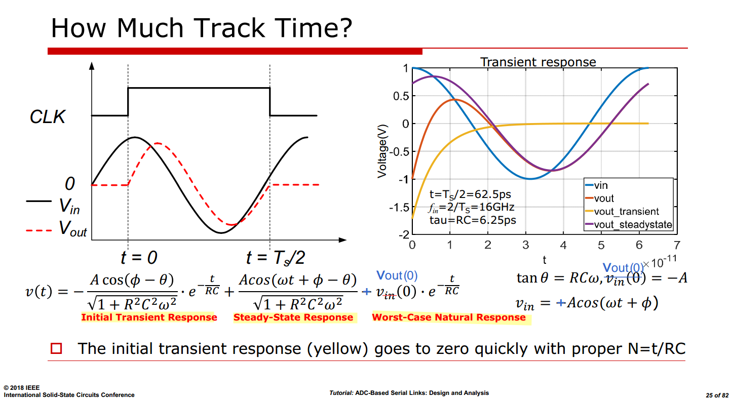
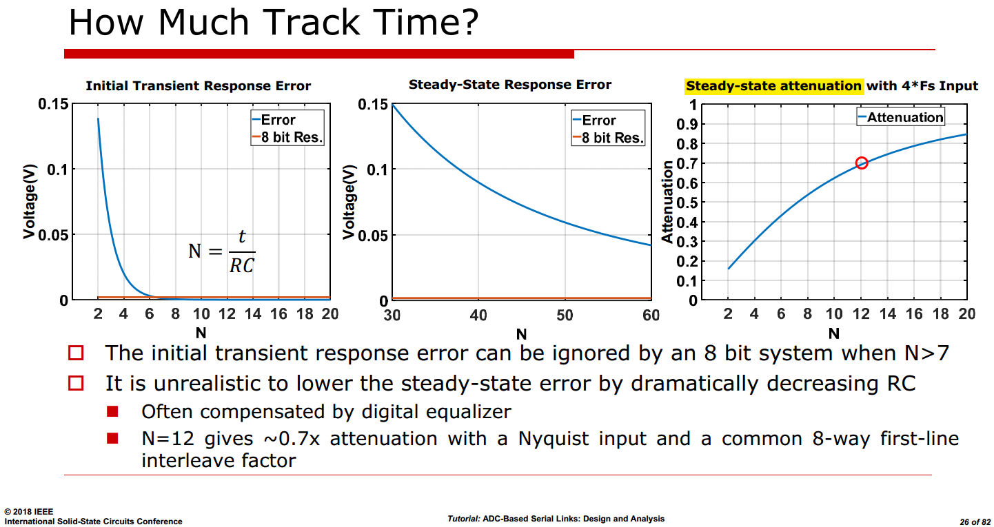
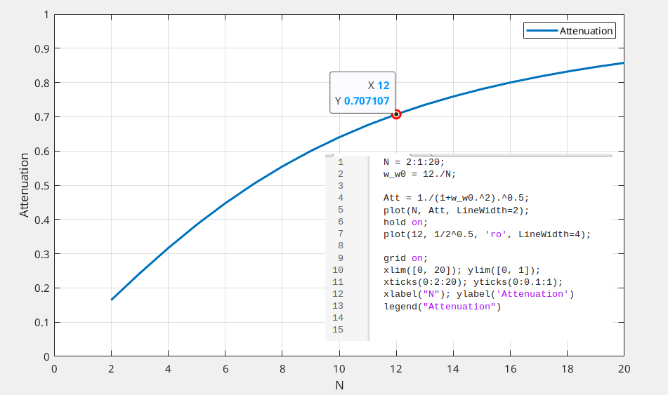
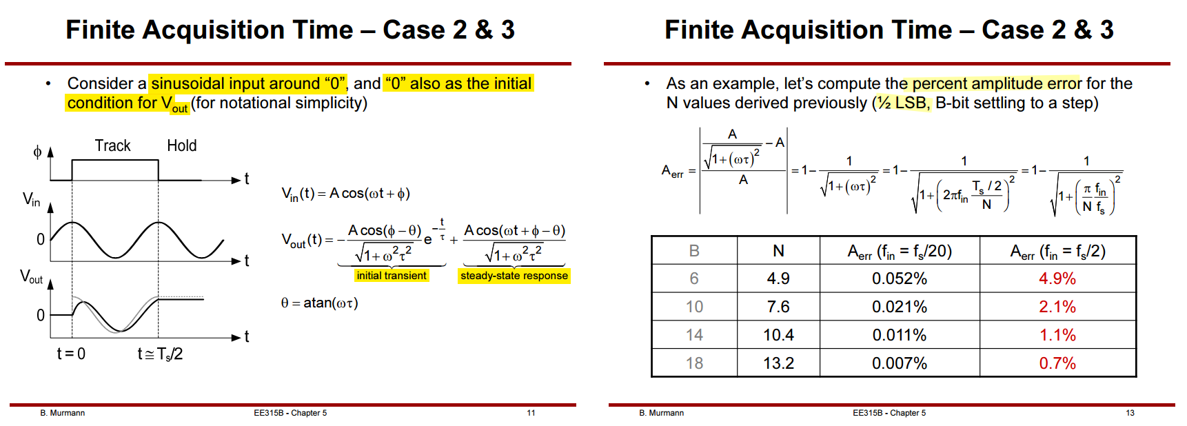
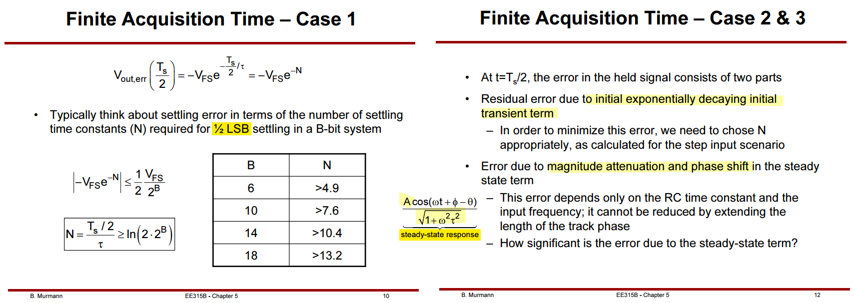
Finite Acquisition Time - Consider a sinusoidal input
\[\begin{align} V_\text{in}(t)=\cos(\omega t+\theta) & \overset{\mathcal{L}}{\Rightarrow} \frac{s\cos \theta-\omega \sin \theta}{s^2+\omega^2} \\ h(t) & \overset{\mathcal{L}}{\Rightarrow} \frac{\frac{1}{\tau}}{s+\frac{1}{\tau}} \end{align}\]
Then,
\[\begin{align} V_\text{out}(s) &= V_\text{in}(s)\cdot H(s) \\ &= \frac{s\cos \theta-\omega \sin \theta}{s^2+\omega^2} \cdot \frac{\frac{1}{\tau}}{s+\frac{1}{\tau}} \\ &= \frac{A}{s+\frac{1}{\tau}} + \frac{Bs+C}{s^2+\omega^2} \end{align}\]
Obtain,
\[ A = -\frac{\cos(\theta - \phi)}{\sqrt{ \omega^2\tau ^2 +1}} \qquad\qquad B = -A \qquad\qquad C = -\frac{\omega \sin(\theta - \phi)}{\sqrt{\omega^2\tau ^2 +1}} \]
That is \[ \boxed{V_\text{out}(s) = -\frac{\cos(\theta - \phi)}{\sqrt{\omega^2\tau ^2 +1}} \frac{1}{s+\frac{1}{\tau}} + \frac{1}{\sqrt{\omega^2\tau ^2 +1}}\frac{s\cos(\theta - \phi) - \omega \sin(\theta - \phi)}{s^2+\omega^2}} \]
where \(\phi = \arctan(\omega \tau)\)
The relation \(V_\text{out}(s) = H(s)\,V_\text{in}(s)\) is the zero-state response only. The transfer function is defined under the assumption \(V_\text{out}(0^-) = 0\), so you can't recover the natural response from it. You have to go back one step, to the differential equation.
For the RC (track) network with \(\tau = RC\):
\[ \tau \dot{V}_\text{out} + V_\text{out} = V_\text{in} \]
Transform with the full derivative rule \(\mathcal{L}\{\dot{V}_\text{out}\} = s V_\text{out}(s) - V_0\), where \(V_0 \equiv V_\text{out}(0^-)\) (the capacitor voltage is continuous, so \(0^-\) and \(0^+\) agree): \[ \tau\big(s V_\text{out}(s) - V_0\big) + V_\text{out}(s) = V_\text{in}(s) \]
\[ \boxed{\;V_\text{out}(s) = \underbrace{\frac{V_\text{in}(s)}{\tau s + 1}}_{\text{zero-state}} + \underbrace{\frac{\tau V_0}{\tau s + 1}}_{\text{zero-input}} = H(s)\,V_\text{in}(s) + \frac{V_0}{s + \frac{1}{\tau}}\;} \]
Then the Complete Laplace Expression is \[ \boxed{V_\text{out}(s) = -\frac{\cos(\theta - \phi)}{\sqrt{\omega^2\tau ^2 +1}} \frac{1}{s+\frac{1}{\tau}} + \frac{1}{\sqrt{\omega^2\tau ^2 +1}}\frac{s\cos(\theta - \phi) - \omega \sin(\theta - \phi)}{s^2+\omega^2} + \frac{V_\text{out}(0)}{s + \frac{1}{\tau}} } \] The Total Time-Domain Solution \[ \boxed{V_{\text{out}}(t) = \underbrace{V_{\text{out}}(0)e^{-\frac{t}{\tau}}}_{\text{Pure Natural Response}} + \underbrace{\frac{1}{\sqrt{\omega^2\tau^2 + 1}} \left[ \cos(\omega t + \theta - \phi) - \cos(\theta - \phi) e^{-\frac{t}{\tau}} \right]}_{\text{Forced Response (Transient + Steady-State)}} } \] And grouped by transient vs. steady-state components: \[ \boxed{V_{\text{out}}(t) = \underbrace{\left[ V_{\text{out}}(0) - \frac{\cos(\theta - \phi)}{\sqrt{\omega^2\tau^2 + 1}} \right] e^{-\frac{t}{\tau}}}_{\text{Total Transient Response}} + \underbrace{\frac{\cos(\omega t + \theta - \phi)}{\sqrt{\omega^2\tau^2 + 1}}}_{\text{Steady-State Response}}} \]
Tracking Nonlinearity
Wei Yu, Subhajit Sen and B. H. Leung, "Distortion analysis of MOS track-and-hold sampling mixers using time-varying Volterra series," in IEEE Transactions on Circuits and Systems II: Analog and Digital Signal Processing, vol. 46, no. 2, pp. 101-113, Feb. 1999 [https://sci-hub.ru/10.1109/82.752910]
B. Murmann, EE315B VLSI-Data-Conversion-Circuits [https://dl.sabzdanesh.com/Electronic/VLSI-Data-Conversion-Circuits_(WWW.SabzElco.IR).pdf]
\[\begin{align} HD_2 &\approx \frac{1}{2}\omega C V_m \frac{\mathcal{d} R_{on}}{\mathcal{d}v_{in}}\bigg\rvert_{v_{in}=0}=\frac{1}{2}\omega C V_m\frac{R_{ON}}{V_{OV}} = \frac{1}{2}\frac{\omega}{\omega_c}\frac{V_m}{V_{OV}} \\ HD_3 &\approx \frac{1}{4}\omega C V_m^2 \frac{\mathcal{d}^2 R_{on}}{\mathcal{d}v_{in}^2}\bigg\rvert_{v_{in}=0}=\frac{1}{4}\omega C V_m^2\frac{R_{ON}}{V_{OV}^2} = \frac{1}{2}\frac{\omega}{\omega_c}\left(\frac{V_m}{V_{OV}}\right)^2 \end{align}\]
where \(V_{OV}=V_{DD}-V_{IN}-V_t\), \(R_{ON}=\frac{1}{\mu C_{ox}W/LV_{OV}}\) and \(\omega_c=1/R_{ON}C\)
Even-order distortion products cancel in perfectly symmetrical circuits; But phase and amplitude imbalances lead to finite \(HD_2\) in practice
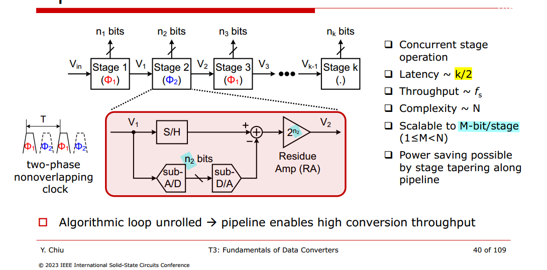
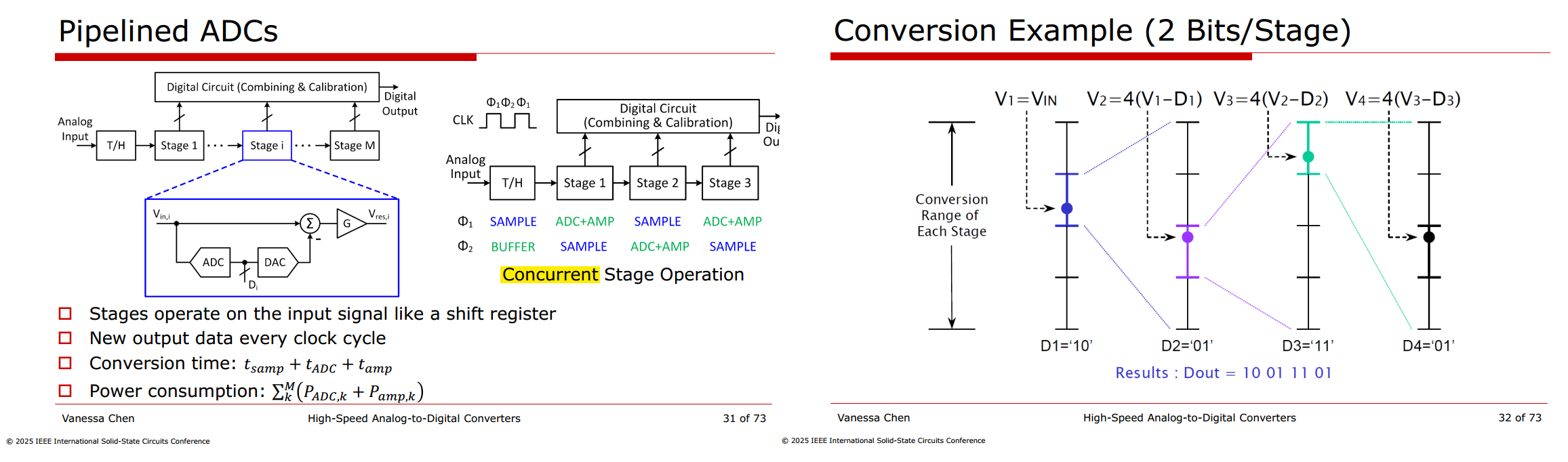
Pipeline ADC
Vishal Saxena, "Pipelined ADC Design - A Tutorial"[https://www.eecis.udel.edu/~vsaxena/courses/ece517/s17/Lecture%20Notes/Pipelined%20ADC%20NonIdealities%20Slides%20v1_0.pdf] [https://www.eecis.udel.edu/~vsaxena/courses/ece517/s17/Lecture%20Notes/Pipelined%20ADC%20Slides%20v1_2.pdf]
Bibhu Datta Sahoo, Analog-to-Digital Converter Design From System Architecture to Transistor-level [http://smdpc2sd.gov.in/downloads/IGF/IGF%201/Analog%20to%20Digital%20Converter%20Design.pdf]
Bibhu Datta Sahoo, Associate Professor, IIT, Kharagpur, [https://youtu.be/HiIWEBAYRJY]
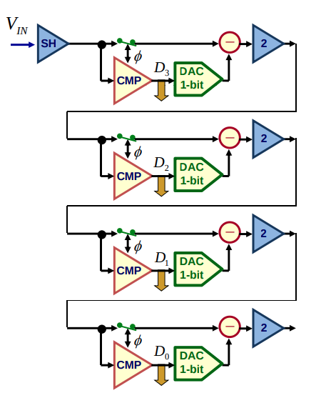
CMP reference voltage is 0.5vref, DAC output is 0.5vref or 0

residual error \[ V_{r,n} = (V_{r,n-1}-\frac{1}{2}b_{n})\cdot 2 \] and \(V_{r,-1}=V_i\) \[ V_{r,n-1} = 2^{n}V_i -\sum_{k=0}^{n-1}2^{n-k-1}b_k = 2^{n}\left(V_i - \sum_{k=0}^{n-1}\frac{b_k}{2^{k+1}}\right) \]
here, \(b_0\) is first stage and MSB
It divides the process into several comparison stages, the number of which is proportional to the number of bits
Due to the pipeline structure of both analog and digital signal path, inter-stage residue amplification is needed which consumes considerable power and limits high speed operation
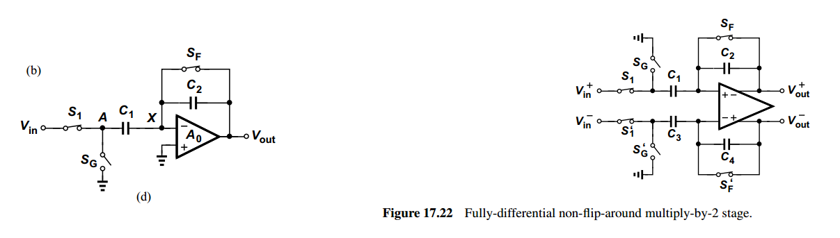
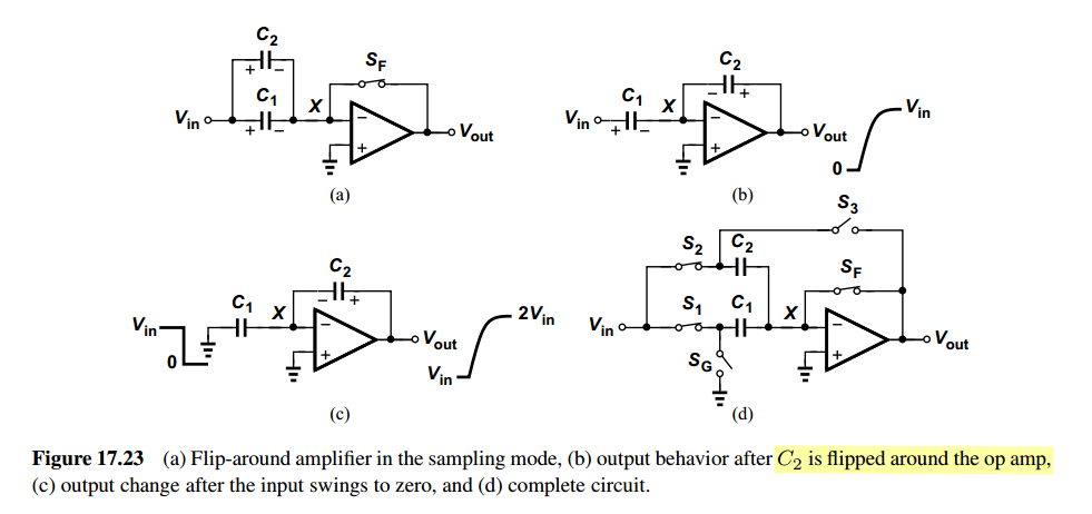
Non-Flip-Around & Flip-Around Amplifier
Non-Flip-Around Amplifier
The amplifier's differential input stays approximately zero after settling; its individual input voltages need not be constant
With matched capacitors, their common-mode contributions cancel when we subtract the two charge-conservation equations
Flip-Around Amplifier
Multiplying DACs (MDAC)
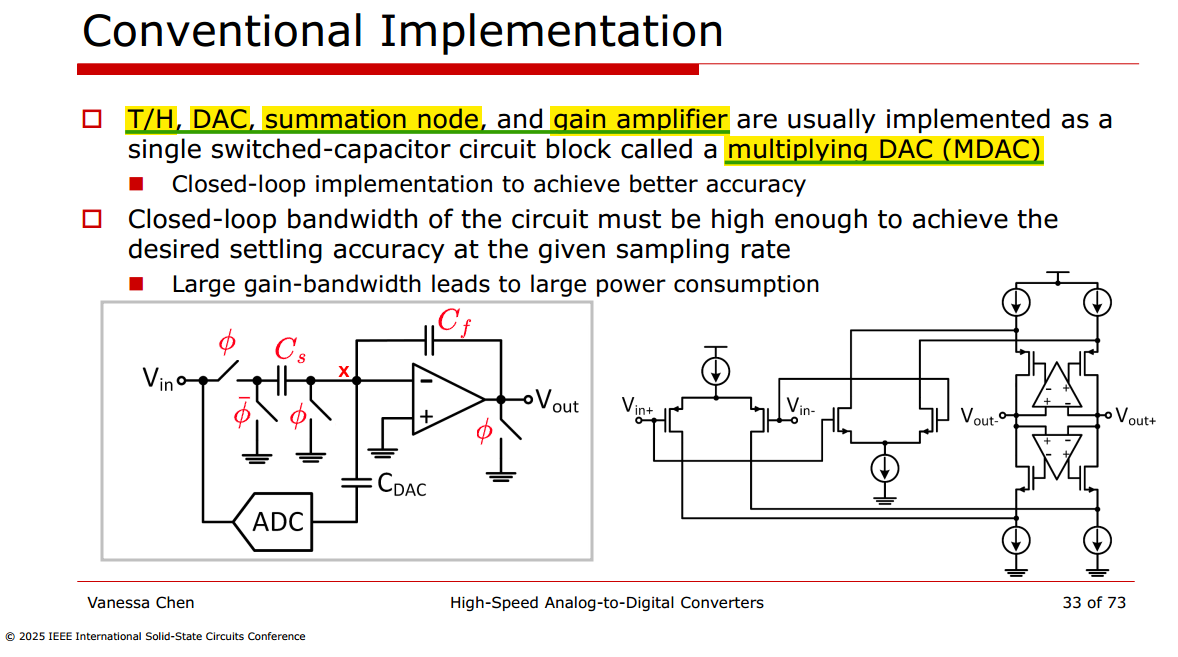
| Connection | Sampling phase | Amplification phase |
|---|---|---|
| (V_{}) to left plate of (C_S) | Closed | Open |
| Left plate of (C_S) to ground | Open | Closed |
| Node (x) to ground | Closed | Open |
| Output to ground | Closed | Open |
Phase 1: sample the input
- \(C_S\) has \(V_{\text{in}}\) on its left plate and 0 V on its right plate, so it stores the input as charge.
- Both ends of \(C_F\) are grounded, resetting its voltage to zero.
- The small ADC samples the same input and determines a digital code.
At the end of sampling:
\[ Q_{x,\text{sample}}=-C_SV_{\text{in}} \]
Phase 2: subtract and amplify
- Switching (C_S)’s left plate from (V_{}) to zero disturbs node (x).
- Switching the DAC bottom plate from zero to (V_D) produces an opposing disturbance.
- The amplifier changes (V_{}), through (C_F), to balance the remaining charge.
After amplification settles, both ends of \(C_S\) are approximately zero:
\[ Q_{x,\text{amp}}=-C_FV_{\text{out}}-C_{\text{DAC}}V_D \]
Equating them:
\[ \boxed{ V_{\text{out}} = \frac{C_S}{C_F}V_{\text{in}} - \frac{C_{\text{DAC}}}{C_F}V_D } \]
If \(C_S=C_{\text{DAC}}\), this becomes:
\[ \boxed{V_{\text{out}}=G(V_{\text{in}}-V_D)}, \qquad G=\frac{C_S}{C_F} \]
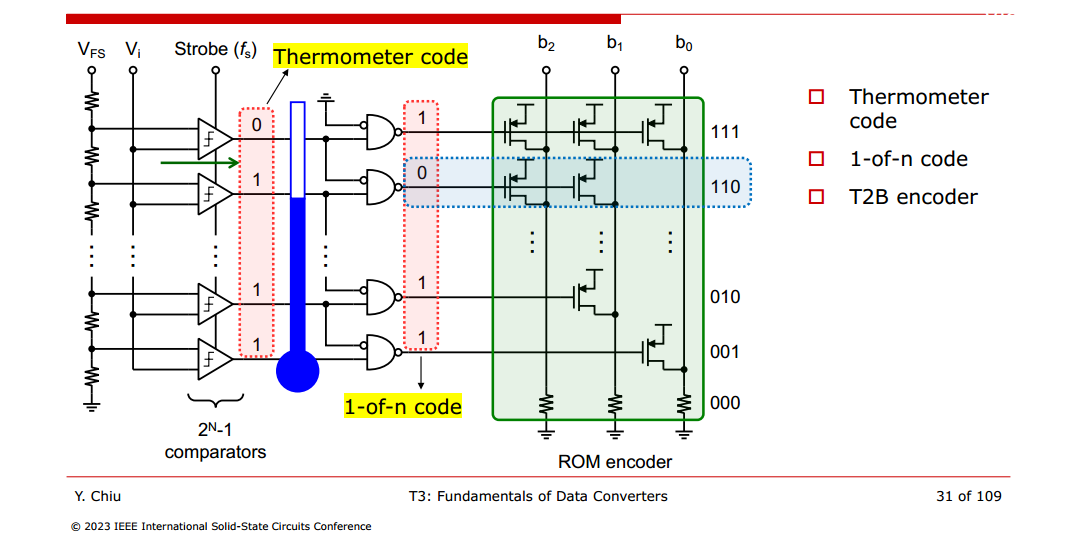
Thermometer to Binary encoder
R-2R & C-2C
B. Razavi, "The R-2R and C-2C Ladders [A Circuit for All Seasons]," in IEEE Solid-State Circuits Magazine, vol. 11, no. 3, pp. 10-15, Summer 2019 [https://www.seas.ucla.edu/brweb/papers/Journals/BR_SSCM_3_2019.pdf]
\(N_b\) bit binary + \(N_t\) bit thermometer DAC

\(N_b\) bit binary can be simplified with Thevenin Equivalent \[ V_B = \sum_{n=0}^{N_b-1} \frac{B_n}{2^{N_b-n}} \] with thermometer code
\[ V_o = V_B\frac{\frac{2R}{2^{N_t}-1}}{\frac{2R}{2^{N_t}-1}+ 2R}+\sum_{n=0}^{2^{N_t}-2}T_n\frac{\frac{2R}{2^{N_t}-1}}{\frac{2R}{2^{N_t}-1}+ 2R} = \frac{V_B}{2^{N_t}} + \frac{\sum_{n=0}^{2^{N_t}-2}T_n}{2^{N_t}} = \sum_{n=0}^{N_b-1} \frac{B_n}{2^{N_t+N_b-n}} + \frac{\sum_{n=0}^{2^{N_t}-2}T_n}{2^{N_t}} \]
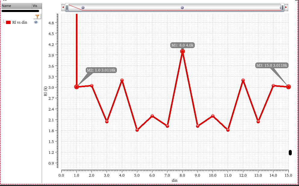
4bit binary R2R DAC with Ru=1kOhm; RVB equivalent R
reference
Maloberti, F. Data Converters. Dordrecht, Netherlands: Springer, 2007.
Ali, Ahmed M. A. High Speed Data Converters. The Institution of Engineering and Technology, 2016.
Razavi B. Analysis and Design of Data Converters. Cambridge University Press; 2025.
Aaron Buchwald, ISSCC2010 T1: "Specifying & Testing ADCs"
Ahmed M. A. Ali. CICC 2018: High Speed Pipelined ADCs: Fundamentals and Variants
John P. Keane, ISSCC2020 T5: "Fundamentals of Time-Interleaved ADCs"
Yun Chiu, ISSCC2023 T3: "Fundamentals of Data Converters" [https://personal.utdallas.edu/~yxc101000/courses/7327/handout/isscc2023_tutorial.pdf]
—, "Design and Calibration Techniques for SAR and Pipeline ADCs" [http://formation-old.in2p3.fr/microelectronique15/IN2P3_ADC.pdf]
—, Radiation-Tolerant SAR ADC Architecture and Digital Calibration Techniques [https://indico.cern.ch/event/385097/attachments/768706/1054353/CERN_May15.pdf]
—, Recent Advances in Multistep Nyquist ADC's [https://www.eecis.udel.edu/~vsaxena/courses/ece614/Handouts/Recent%20Advances%20in%20Nyquist%20rate%20ADCs.pdf]
Aaron Buchwald, ISSCC 2008 T2 Pipelined A/D Converters: The Basics
Yohan Frans, CICC2019 ES3-3- "ADC-based Wireline Transceivers" [pdf]
Samuel Palermo, ISSCC 2018 T10: ADC-Based Serial Links: Design and Analysis
Jan Mulder Broadcom. ISSCC2015 T5: High-Speed Current-Steering DACs
Zhang, Milin, Zhihua Wang, Jan van der Spiegel and Franco Maloberti. "Advanced Tutorial on Analog Circuit Design." (2023)
V. Chen, "Tutorial: High-Speed Analog-to-Digital Converters," 2025 IEEE International Solid-State Circuits Conference (ISSCC), San Francisco, CA, USA, 2025, pp. 1-1, doi: 10.1109/ISSCC49661.2025.11076112.
S. Su, "Principles and Practices of High-Speed DAC Design: From Conversion Fundamentals to Layout-Aware Implementation," in IEEE Solid-State Circuits Magazine, vol. 18, no. 3, pp. 26-43, Summer 2026, doi: 10.1109/MSSC.2026.3704105
M. Gu, Y. Tao, Y. Zhong, L. Jie and N. Sun, "Timing-Skew Calibration Techniques in Time-Interleaved ADCs," in IEEE Open Journal of the Solid-State Circuits Society [https://ieeexplore.ieee.org/stamp/stamp.jsp?tp=&arnumber=10804623]
everynanocounts. Memos on FFT With Windowing. URL: https://a2d2ic.wordpress.com/2018/02/01/memos-on-fft-with-windowing/
How to choose FFT depth for ADC performance analysis (SINAD, ENOB). URL:https://dsp.stackexchange.com/a/38201
Computation of Effective Number of Bits, Signal to Noise Ratio, & Signal to Noise & Distortion Ratio Using FFT. URL:https://cdn.teledynelecroy.com/files/appnotes/computation_of_effective_no_bits.pdf
Kester, Walt. (2009). Understand SINAD, ENOB, SNR, THD, THD + N, and SFDR so You Don't Get Lost in the Noise Floor. URL:https://www.analog.com/media/en/training-seminars/tutorials/MT-003.pdf
T. C. Hofner: Dynamic ADC testing part I. Defining and testing dynamic ADC parameters, Microwaves & RF, 2000, vol. 39, no. 11, pp. 75-84,162
—: Dynamic ADC testing part 2. Measuring and evaluating dynamic line parameters, Microwaves & RF, 2000, vol. 39, no. 13, pp. 78-94
AN9675: A Tutorial in Coherent and Windowed Sampling with A/D Converters https://www.renesas.com/us/en/document/apn/an9675-tutorial-coherent-and-windowed-sampling-ad-converters
APPLICATION NOTE 3190: Coherent Sampling Calculator (CSC) https://www.stg-maximintegrated.com/en/design/technical-documents/app-notes/3/3190.html
Coherent Sampling (Very Brief and Simple) https://www.dsprelated.com/thread/469/coherent-sampling-very-brief-and-simple
Signal Chain Basics #160: Making sense of coherent and noncoherent sampling in data-converter testing https://www.planetanalog.com/signal-chain-basics-160-making-sense-of-coherent-and-noncoherent-sampling-in-data-converter-testing/
Signal Chain Basics #104: Understanding noise in ADCs https://www.planetanalog.com/signal-chain-basics-part-104-understanding-noise-in-adcs/
Signal Chain Basics #101: ENOB Degradation Analysis Over Frequency Due to Jitter https://www.planetanalog.com/signal-chain-basics-part-101-enob-degradation-analysis-over-frequency-due-to-jitter/
Clock jitter analyzed in the time domain, Part 1, Texas Instruments Analog Applications Journal (slyt379), Aug 2010 https://www.ti.com/lit/an/slyt379/slyt379.pdf
Clock jitter analyzed in the time domain, Part 2 https://www.ti.com/lit/slyt389
Measurement of Total Harmonic Distortion and Its Related Parameters using Multi-Instrument [pdf]
Application Note AN-4: Understanding Data Converters' Frequency Domain Specifications [pdf]
Belleman, J. (2008). From analog to digital. 10.5170/CERN-2008-003.131. [pdf]
HandWiki. Coherent sampling [link]
Luis Chioye, TI. Leverage coherent sampling and FFT windows when evaluating SAR ADCs (Part 1) [link]
Coherent Sampling vs. Window Sampling | Analog Devices https://www.analog.com/en/technical-articles/coherent-sampling-vs-window-sampling.html
Understanding Effective Number of Bits https://robustcircuitdesign.com/signal-chain-explorer/understanding-effective-number-of-bits/
ADC Input Noise: The Good, The Bad, and The Ugly. Is No Noise Good Noise? [https://www.analog.com/en/resources/analog-dialogue/articles/adc-input-noise.html]
Walt Kester, Taking the Mystery out of the Infamous Formula, "SNR = 6.02N + 1.76dB," and Why You Should Care [https://www.analog.com/media/en/training-seminars/tutorials/MT-001.pdf]
Dan Boschen, "How to choose FFT depth for ADC performance analysis (SINAD, ENOB)", [https://dsp.stackexchange.com/a/38201]
B. Razavi, "A Tale of Two ADCs - Pipelined Versus SAR" IEEE Solid-State Circuits Magazine, Volume. 7, Issue. 30, pp. 38-46, Summer 2015 [https://www.seas.ucla.edu/brweb/papers/Journals/BRSummer15ADC.pdf)]
Dr. Tai-Haur Kuo (郭泰豪 教授) Analog IC Design (類比積體電路設計) [http://msic.ee.ncku.edu.tw/course/aic/aic.html]
Converter Passion for data-converter professionals sharing thoughts on ADCs and DACs [https://converterpassion.wordpress.com/]
Boris Murmann, EE315B VLSI Data Conversion Circuits, Autumn 2013
MPScholar Analog-to-Digital Converters (ADCs) [https://www.monolithicpower.com/en/learning/mpscholar/analog-to-digital-converters]
tomverbeure. List of Analog Devices Tutorials [https://tomverbeure.github.io/2021/02/15/Analog-Devices-Tutorials.html]