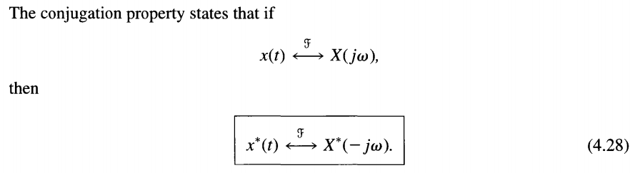
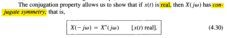
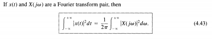
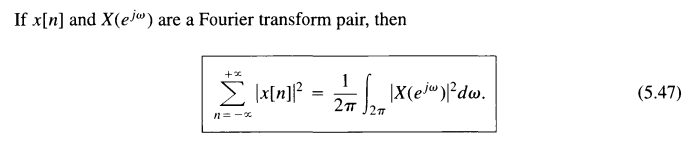
Fourier Transform
discrete-time frequency: \(\hat{\omega}=\omega T_s\), units are radians per sample
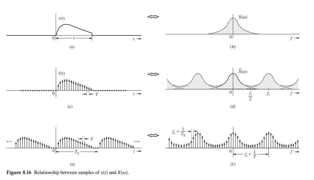
Below diagram show the windowing effect and sampling

For general window function, we know \(W(e^{j\hat{\omega}})=\frac{1}{T_s}W_c(j\frac{\hat\omega}{T_s})\),
\[ \frac{W_c(j\frac{\hat{\omega}}{T_s})X_c(j\frac{\hat{\omega}}{T_s})}{T_s}\cdot \frac{1}{2\pi} = \frac{T_sW(e^{j\hat{\omega}})X_c(j\frac{\hat\omega}{T_s})}{T_s}\cdot \frac{1}{2\pi}=W(e^{j\hat{\omega}})X_c(j\frac{\hat\omega}{T_s})\cdot \frac{1}{2\pi} \overset{\hat{\omega}=0}{\Longrightarrow} \sum_{n=-N_w}^{+N_w}w[n] \cdot X_c(j\omega)\cdot \frac{1}{2\pi} \]
e.g. \(\frac{W_c(j\omega|\omega=0)}{T_s} = N\) for Rectangular Window, shown in above figure
warmup
| Continuous-time signals \(x_c(t)\) | Discrete-time signals \(x[n]\) | |
|---|---|---|
| Aperiodic signals | Continuous Fourier transform | Discrete-time Fourier transform |
| Periodic signals | Fourier series | Discrete Fourier transform |
Continuous Time Fourier Series (CTFS)
\[\begin{align} a_k &= \frac{1}{T}\int_T x(t)e^{-jk(2\pi/T)) t}dt \\ x(t) &= \sum_{k=-\infty}^{+\infty}a_ke^{jk(2\pi/T) t} \end{align}\]
Continuous-Time Fourier transform (CTFT)
\[\begin{align} X(j\omega) &=\int_{-\infty}^{+\infty}x(t)e^{-j\omega t}dt \\ x(t)&= \frac{1}{2\pi}\int_{-\infty}^{+\infty}X(j\omega)e^{j\omega t}d\omega \end{align}\]
[https://www.rose-hulman.edu/class/ee/yoder/ece380/Handouts/Fourier%20Transform%20Tables%20w.pdf]
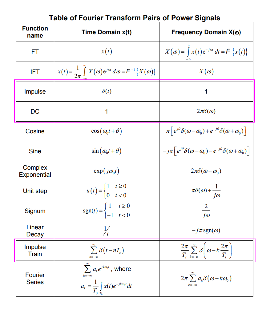
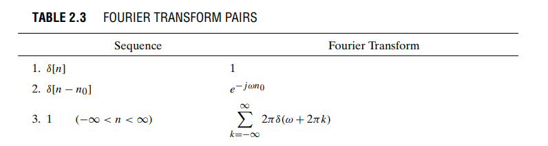
Discrete-Time Fourier Transform (DTFT)
\[\begin{align} X(e^{j\hat{\omega}}) &=\sum_{n=-\infty}^{+\infty}x[n]e^{-j\hat{\omega} n} \\ x[n] &= \frac{1}{2\pi}\int_{2\pi}X(e^{j\hat{\omega}})e^{j\hat{\omega} n}d\hat{\omega} \end{align}\]
DTFT is defined for infinitely long signals as well as finite-length signal
DTFT is continuous in the frequency domain
We could verify that is the correct inverse DTFT relation by substituting the definition of the DTFT and rearranging terms
Discrete-Time Fourier Series (DTFS)
TODO 📅
Discrete Fourier Series (DFS)
TODO 📅
Discrete Fourier Transform (DFT)
Two steps are needed to change the DTFT sum into a computable form:
- the continuous frequency variable \(\hat{\omega}\) must be sampled
- the limits on the DTFT sum must be finite
\[\begin{align} X[k] &= \sum_{n=0}^{N-1}x[n]e^{-j(2\pi/N)kn}\space\space\space k=0,1,...,N-1 \\ x[n] &= \frac{1}{N}\sum_{k=0}^{N-1}X[k]e^{j(2\pi/N)kn} \space\space\space n=0,1,...,N-1 \end{align}\]
Part of the proof is given by the following step:
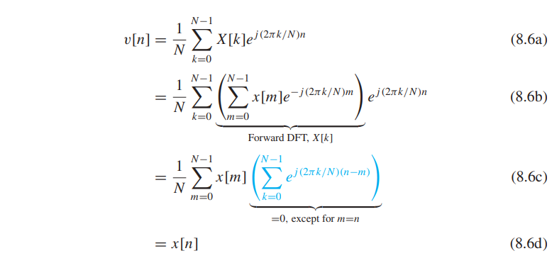
DFT \(X[k]\) is a sampled version of the DTFT \(X(e^{j\hat{\omega}})\), where \(\hat{\omega_k} = \frac{2\pi k}{N}\)
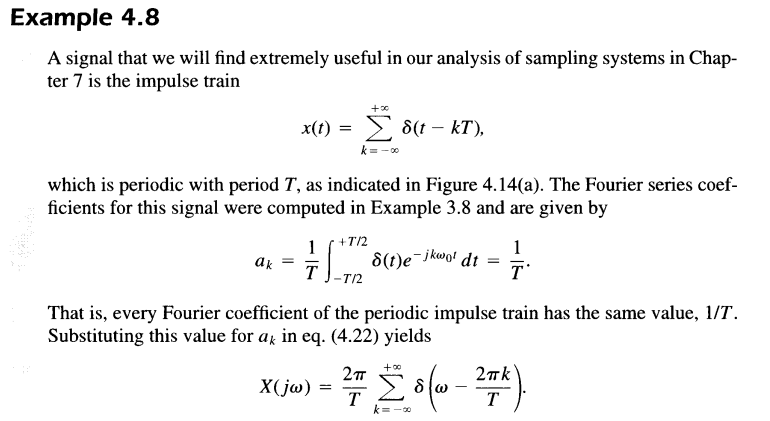
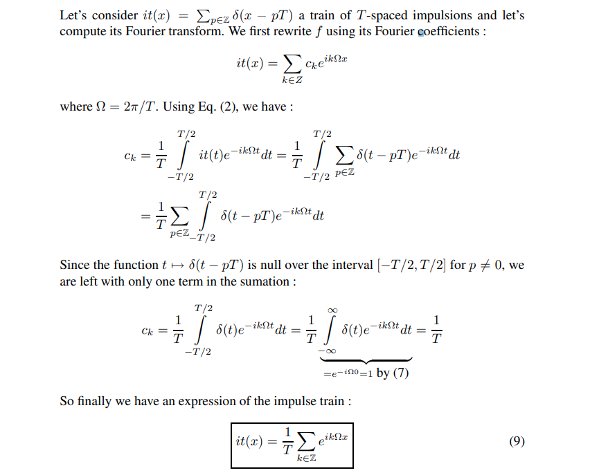
impulse train
CTFT:
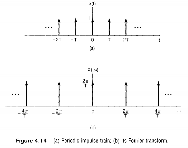
using time-sampling property

DTFT:
Given \(x[n]=\sum_{k=-\infty}^{\infty}\delta(n-k)\)
\[\begin{align} X(e^{j\hat{\omega}}) &= X_s(j\frac{\hat{\omega}}{T}) \\ &= \frac{2\pi}{T}\sum_{k=-\infty}^{\infty}\delta(\frac{\hat{\omega}}{T}-\frac{2\pi k}{T}) \\ &= \frac{2\pi}{T}\sum_{k=-\infty}^{\infty}T\delta(\hat{\omega}-2\pi k) \\ &= 2\pi\sum_{k=-\infty}^{\infty}\delta(\hat{\omega}-2\pi k) \end{align}\]
Fourier series of impulse train
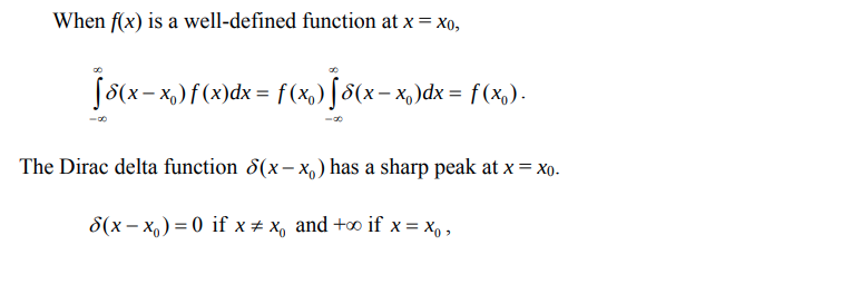
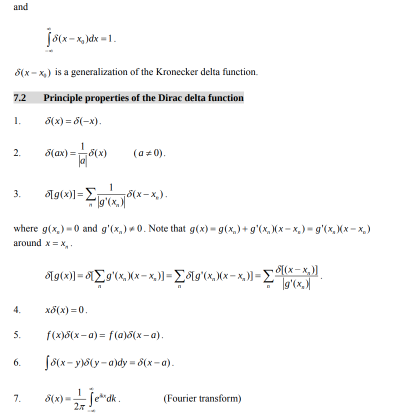
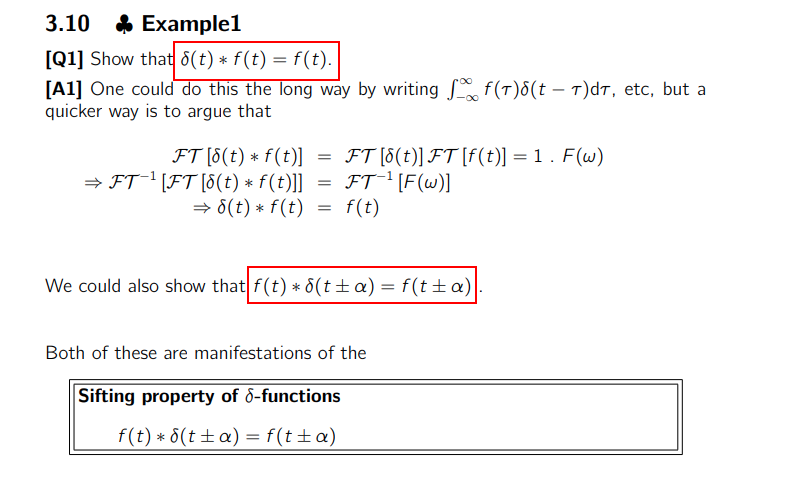
Dirac delta (impulse) function
[https://bingweb.binghamton.edu/~suzuki/Math-Physics/LN-7_Dirac_delta_function.pdf]
Topic 3 The \(\delta\)-function & convolution. Impulse response & Transfer function [https://www.robots.ox.ac.uk/~dwm/Courses/2TF_2011/2TF-N3.pdf]
impulse scaling
\[ \delta(\alpha t)= \frac{1}{\alpha}\delta( t) \]
where \(\alpha\) is scaling ratio
Multiplication
aka Modulation or Windowing Theorem
CTFT: \[ x_1(t)x_2(t)\overset{FT}{\longrightarrow}\frac{1}{2\pi}X_1(\omega)*X_2(\omega) \]
DTFT:
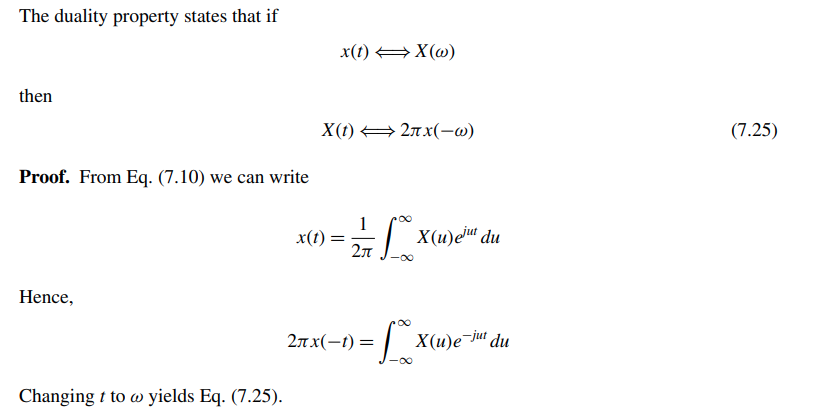
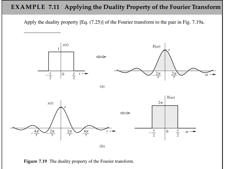
Duality
Conjugate Symmetry
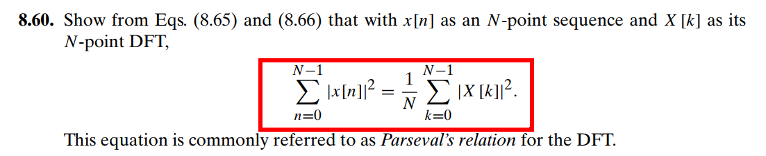
Parseval's Relation
CTFT:
DTFT:
DFT:
Eigenfunctions & frequency response
Complex exponentials are eigenfunctions of LTI systems, that is,
continuous time: \(e^{j\omega t}\to H(j\omega)e^{j\omega t}\)
discrete time: \(e^{j\hat{\omega}n} \to H(e^{j\hat{\omega}})e^{j\hat{\omega}n}\)
where \(H(j\omega)\), \(H(e^{j\hat{\omega}})\) is frequency response of continuous-time systems and discrete-time systems, which is the function of \(\omega\) and \(\hat{\omega}\) \[\begin{align} H(j\omega) &= \int_{-\infty}^{+\infty}h(t)e^{-j\omega t}dt \\ \\ H(e^{j\hat{\omega}}) &= \sum_{n=-\infty}^{+\infty}h[n]e^{-j\hat{\omega} n} \end{align}\]
The frequency response of discrete-time LTI systems is always a periodic function of the frequency variable \(\hat{\omega}\) with period \(2\pi\)
Sampling Theorem
time-sampling theorem: applies to bandlimited signals
spectral sampling theorem: applies to timelimited signals
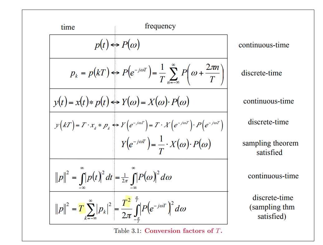
Aliasing
The frequencies \(f_{\text{sig}}\) and \(Nf_s \pm f_{\text{sig}}\) (\(N\) integer), are indistinguishable in the discrete time domain.
Given below sequence \[ X[n] =A e^{j\omega T_s n} \]
- \(kf_s + \Delta f\)
\[\begin{align} x[n] &= Ae^{j\left( kf_s+\Delta f \right)2\pi T_sn} + Ae^{j\left( -kf_s-\Delta f \right)2\pi T_sn} \\ &= Ae^{j\Delta f\cdot 2\pi T_sn} + Ae^{-j\Delta f\cdot 2\pi T_sn} \end{align}\]
- \(kf_s - \Delta f\)
\[\begin{align} x[n] &= Ae^{j\left( kf_s-\Delta f \right)2\pi T_sn} + Ae^{j\left( -kf_s+\Delta f \right)2\pi T_sn} \\ &= Ae^{-j\Delta f\cdot 2\pi T_sn} + Ae^{j\Delta f\cdot 2\pi T_sn} \end{align}\]
complex signal
\[\begin{align} A e^{j(\omega_s + \Delta \omega) T_s n} &= A e^{j(k\omega_s + \Delta \omega) T_s n} \\ A e^{j(\omega_s - \Delta \omega) T_s n} &= A e^{j(k\omega_s - \Delta \omega) T_s n} \end{align}\]

CTFS & CTFT
Fourier transform of a periodic signal with Fourier series coefficients \(\{a_k\}\) can be interpreted as a train of impulses occurring at the harmonically related frequencies and for which the area of the impulse at the \(k\)th harmonic frequency \(k\omega_0\) is \(2\pi\) times the \(k\)th Fourier series coefficient \(a_k\)
inverse CTFT & inverse DTFT
| time domain | frequency domain | |
|---|---|---|
| inverse CTFT | \(\delta(t)\) | \(\int_{\infty}d\omega\) |
| inverse DTFT | \(\delta[n]\) | \(\int_{2\pi}d\hat{\omega}\) |
inverse CTFT shall integral from \(-\infty\) to \(+\infty\) to obtain \(\delta(t)\) in time domain, e.g., \(x_s(t)\) impulse train
spectral sampling
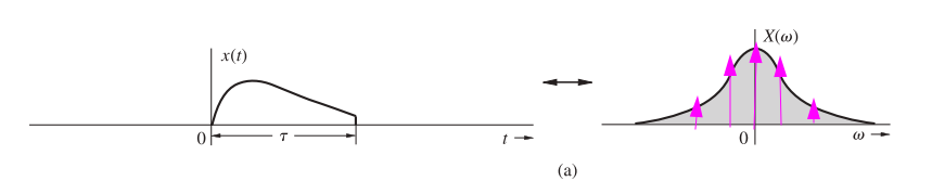
spectral sampling by \(\omega_0\), and \(\frac{2\pi}{\omega_0} \gt \tau\) \[ X_{n\omega_0}(\omega) = \sum_{n=-\infty}^{\infty}X(n\omega_0)\delta(\omega - n\omega_0) \] Periodic repetition of \(x(t)\) is \[ x_{n\omega_0}(t) = \frac{1}{\omega_0}\sum_{n=-\infty}^{\infty}x(t -n\frac{2\pi}{\omega_0})=\frac{T_0}{2\pi}\sum_{n=-\infty}^{\infty}x(t -nT_0) \]
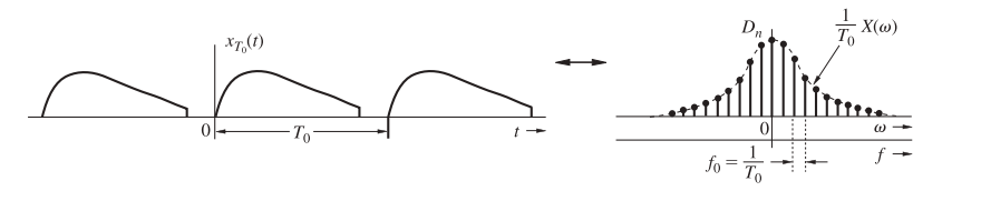
Then, if \(x_{T_0} (t)\), a periodic signal formed by repeating \(x(t)\) every \(T_0\) seconds (\(T_0 \gt \tau\)), its CTFT is \[ X_{T_0}(\omega) = \frac{2\pi}{T_0} \cdot X_{n\omega_0}(\omega) = \frac{2\pi}{T_0}\sum_{n=-\infty}^{\infty}X(n\omega_0)\delta(\omega - n\omega_0) \] Then \(x_{T_0} (t)\) can be expressed with inverse CTFT as \[\begin{align} x_{T_0} (t) &= \frac{1}{2\pi}\int_{-\infty}^{\infty}X_{T_0}(\omega)e^{j\omega t}d\omega \\ &= \frac{1}{T_0}\sum_{n=-\infty}^{\infty}X(n\omega_0)e^{jn\omega_0 t} =\sum_{n=-\infty}^{\infty}\frac{1}{T_0}X(n\omega_0)e^{jn\omega_0 t} \end{align}\]
i.e. the coefficients of the Fourier series for \(x_{T_0} (t)\) is \(D_n =\frac{1}{T_0}X(n\omega_0)\)
alternative method by direct Fourier series
Why DFT ?
We can use DFT to compute DTFT samples and CTFT samples
\[ \overline{x}(t) = \sum_{n=0}^{N_0-1}x(nT)\delta(t-nT) \] applying the Fourier transform yieds \[ \overline{X}(\omega) = \sum_{n=0}^{N_0-1}x[n]e^{-jn\omega T} \] But \(\overline{X}(\omega)\), the Fourier transform of \(\overline{x}(t)\) is \(X(\omega)/T\), assuming negligible aliasing. Hence, \[ X(\omega) = T\overline{X}(\omega) = T\sum_{n=0}^{N_0-1}x[n]e^{-jn\omega T} \] and \[ X(k\omega_0) = T\sum_{n=0}^{N_0-1}x[n]e^{-jn k\omega_0 T} \] with \(\hat{\omega}_0 = \omega_0 T\) \[ X(k\omega_0) = T\sum_{n=0}^{N_0-1}x[n]e^{-jn k\hat{\omega}_0} \] i.e. the relationship between CTFT and DFT is \(X(k\omega_0) = T\cdot X[k]\), DFT is a tool for computing the samples of CTFT
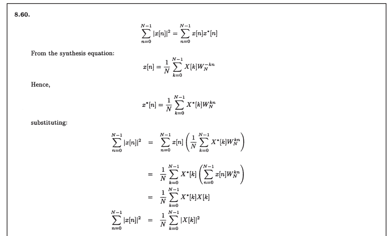
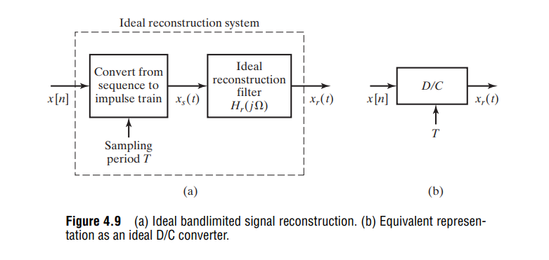
C/D
Sampling with a periodic impulse train, followed by conversion to a discrete-time sequence
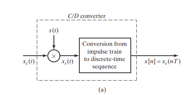
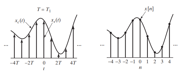
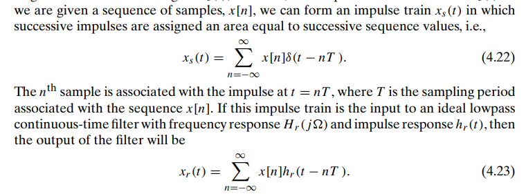
The periodic impulse train is \[ s(t) = \sum_{n=-\infty}^{\infty}\delta(t-nT) \] \(x_s(t)\) can be expressed as \[ x_s(t) = \sum_{n=-\infty}^{\infty}x_c(nT)\delta(t-nT) \] i.e., the size (area) of the impulse at sample time \(nT\) is equal to the value of the continuous-time signal at that time.
\(x_s(t)\) is, in a sense, a continuous-time signal (specifically, an impulse train)
samples of \(x_c(t)\) are represented by finite numbers in \(x[n]\) rather than as the areas of impulses, as with \(x_s(t)\)
Frequency-Domain Representation of Sampling
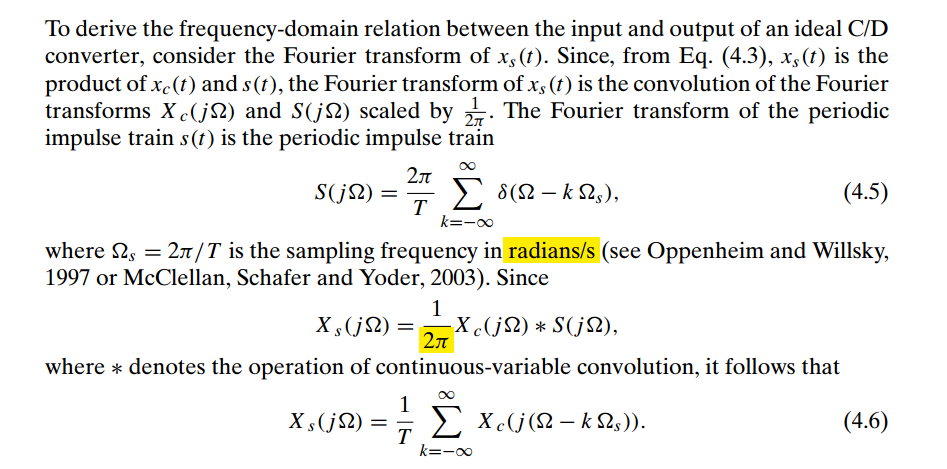
The relationship between the Fourier transforms of the input and the output of the impulse train modulator \[ X_s(j\omega) = \frac{1}{T}\sum_{k=-\infty}^{\infty}X_c(j(\omega -k\omega_s)) \] where \(\omega_s\) is the sampling frequency in radians/s
\(X(e^{j\hat{\omega}})\), the discrete-time Fourier transform (DTFT) of the sequence \(x[n]\), in terms of \(X_s(j\omega)\) and \(X_c(j\omega)\)
| continuous-time Fourier transform | discrete-time Fourier transform |
|---|---|
| \(x_s(t) = \sum_{n=-\infty}^{\infty}x_c(nT)\delta(t-nT)\) | \(x[n]=x_c(nT)\) |
| \(X_s(j\omega)=\sum_{n=-\infty}^{\infty}x_c(nT)e^{-j\omega Tn}\) | \(X(e^{j\hat{\omega}})=\sum_{n=-\infty}^{\infty}x_c(nT)e^{-j\hat{\omega} n}\) |
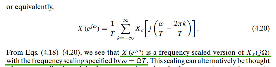
\[ X(e^{j\omega T}) = \frac{1}{T}\sum_{k=-\infty}^{\infty}X_c(j(\omega-k\omega_s)) \] or equivalently, \[ X(e^{j\hat{\omega}}) = \frac{1}{T}\sum_{k=-\infty}^{\infty}X_c(j(\frac{\hat{\omega}}{T}-\frac{2\pi k}{T})) \]
\(X(e^{j\hat{\omega}})\) is a frequency-scaled version of \(X_s(j\omega)\) with the frequency scaling specified by \(\hat{\omega} =\omega T\)
Ref. 9.5 DTFT connection with the CTFT
Here, \(\Omega = \omega T\)
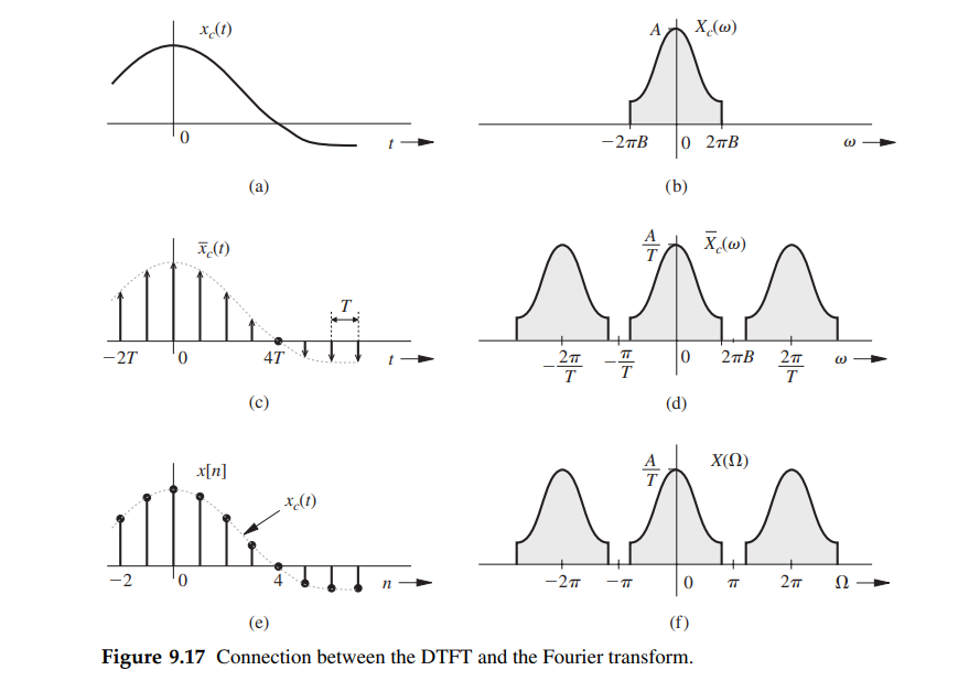
The factor \(\frac{1}{T}\) in \(X(e^{j\hat{\omega}})\) is misleading, actually \(x[n]\) is not scaled by \(\frac{1}{T}\) once taking \(\hat{\omega}\) variable of integration into account \[\begin{align} x_r[n] &= \frac{1}{2\pi} \int_{2\pi}X(e^{j\hat{\omega}})e^{j\hat{\omega} n}d\hat{\omega} \\ &= \frac{1}{2\pi}\int_{2\pi}\frac{1}{T}\sum_{k=-\infty}^{+\infty}X_c \left[ j\left(\frac{\hat{\omega}}{T} - \frac{2\pi k}{T}\right)\right] e^{j\hat{\omega} n}d\hat{\omega} \\ &\approx \frac{1}{2\pi}\frac{1}{T}\int_{2\pi}X_c (\frac{\hat{\omega}}{T} ) e^{j\hat{\omega} n} d\hat{\omega} \\ &=\frac{1}{2\pi} \frac{1}{T}\int_{2\pi} \left[ \int_{\infty}X_c(\Phi)\delta (\Phi - \frac{\hat{\omega}}{T} )d\Phi \right] e^{j\hat{\omega} n} d\hat{\omega} \\ &=\frac{1}{2\pi} \frac{1}{T} \int_{\infty}X_c(\Phi)d\Phi \int_{2\pi}\delta (\Phi - \frac{\hat{\omega}}{T} )e^{j\hat{\omega} n} d\hat{\omega} \\ &=\frac{1}{2\pi} \frac{1}{T} \int_{\infty}X_c(\Phi)d\Phi \int_{2\pi}T\cdot \delta (\Phi T - \hat{\omega} )e^{j\hat{\omega} n} d\hat{\omega} \\ &=\frac{1}{2\pi} \int_{\infty}X_c(\Phi) e^{j\Phi T n}d\Phi \end{align}\]
That is \[\begin{align} x_r[n] &= \frac{1}{2\pi}\int_{2\pi} \frac{1}{T}X_c (\frac{\hat{\omega}}{T} ) e^{j\hat{\omega} n} d\hat{\omega} \\ &= \frac{1}{2\pi} \int_{\infty}X_c(\omega) e^{j\omega T n}d\omega \tag{31} \end{align}\]
assuming Nyquist–Shannon sampling theorem is met
\[\begin{align} x_r[n] &= \frac{1}{2\pi} \int_{\infty}X_c(\omega) e^{j\omega T n}d\omega \\ &= \frac{1}{2\pi} \int_{\infty}X_c(\omega) e^{j\omega t_n}d\omega \\ &= x_c(t_n) \end{align}\]
where \(t_n = T n\), then \(x_r[n] = x_c(nT)\)
Assuming \(x_c(t) = \cos(\omega_0 t)\), \(x_s(t)= \sum_{n=-\infty}^{\infty}x_c(nT)\delta(t-nT)\) and \(x[n]=x_c(nT)\), that is \[\begin{align} x_c(t) & = \cos(\omega_0 t) \\ x_s(t) &= \sum_{n=-\infty}^{\infty}\cos(\omega_0 nT)\delta(t-nT) \\ x[n] &= \cos(\omega_0 nT) \end{align}\]
\(X_c(j\omega)\), the Fourier Transform of \(x_c(t)\) \[ X_c(j\omega) = \pi[\delta(\omega - \omega_0) + \delta(\omega + \omega_0)] \]
\(X(e^{j\hat{\omega}})\), the the discrete-time Fourier transform (DTFT) of the sequence \(x[n]\) \[ X(e^{j\hat{\omega}}) =\sum_{k=-\infty}^{+\infty}\pi[\delta(\hat{\omega} - \hat{\omega}_0-2\pi k) + \delta(\hat{\omega} + \hat{\omega}_0-2\pi k)] \]
\(X_s(j\omega)\), the Fourier Transform of \(x_s(t)\) \[ X_s(j\omega)= \frac{1}{T}\sum_{k=-\infty}^{+\infty}\pi[\delta(\omega - \omega_0-k\omega_s) + \delta(\omega + \omega_0-k\omega_s)] \]
Express \(X(e^{j\hat{\omega}})\) in terms of \(X_s(j\omega)\) and \(X_c(j\omega)\) \[ X(e^{j\hat{\omega}}) = \frac{1}{T}\sum_{k=-\infty}^{+\infty}\pi[\delta(\frac{\hat{\omega}}{T} - \omega_0-k\omega_s) + \delta(\frac{\hat{\omega}}{T} + \omega_0-k\omega_s)] \] Inverse \(X(e^{j\hat{\omega}})\) \[\begin{align} x_r[n] &= \frac{1}{2\pi} \int_{2\pi}X(e^{j\hat{\omega}}) e^{j\hat{\omega} n} d\hat{\omega} \\ &= \frac{1}{2\pi}\int_{2\pi} \pi[\delta(\frac{\hat{\omega}}{T} - \omega_0) + \delta(\frac{\hat{\omega}}{T} + \omega_0)]e^{j\hat{\omega} n} d\frac{\hat{\omega}}{T} \\ &= \frac{1}{2\pi}\int_{2\pi} \pi[\delta(\frac{\hat{\omega}}{T} - \omega_0)e^{j\hat{\omega}_0 n} + \delta(\frac{\hat{\omega}}{T} + \omega_0)e^{-j\hat{\omega}_0 n}] d\frac{\hat{\omega}}{T} \\ &= \frac{1}{2}[ e^{j\hat{\omega}_0 n}\int_{2\pi} [\delta(\frac{\hat{\omega}}{T} - \omega_0)d\frac{\hat{\omega}}{T} + e^{-j\hat{\omega}_0 n}\int_{2\pi} [\delta(\frac{\hat{\omega}}{T} + \omega_0)d\frac{\hat{\omega}}{T}] \\ &= \frac{1}{2}[ e^{j\hat{\omega}_0 n} + e^{-j\hat{\omega}_0 n} ] \\ &= \cos(\hat{\omega}_0 n) \end{align}\]
or follow EQ.(31)
\[\begin{align} x_r[n] &= \frac{1}{2\pi} \int_{\infty}X_c(\omega) e^{j\omega T n}d\omega \\ &= \frac{1}{2\pi} \int_{\infty} \pi[\delta(\omega - \omega_0) + \delta(\omega + \omega_0)]e^{j\omega T n}d\omega \\ &= \frac{1}{2}(e^{j\omega_0 T n}+e^{-j\omega_0 T n}) \\ &= \cos(\hat{\omega}_0 n) \end{align}\]
where \(\hat{\omega}_0 = \omega_0 T\)
impulse train sampling & impulse sequence
if \(x_c(t) = e^{j\Omega_0t}\), thus \(X_c (j\Omega) = A\delta(\Omega - \Omega_0)\)
Then \[ X_s (j\Omega) = \frac{A}{T_s}\sum_k \delta(\Omega -\Omega_0 - k\Omega_s) \]
DTFT of \(x[n]\) \[\begin{align} X(e^{j\omega}) &= \frac{1}{T_s} \sum_k X_c\left[j(\frac{\omega}{T_s}-\frac{2\pi k}{T_s})\right] \\ &= \frac{A}{T_s} \sum_k \delta(\frac{\omega}{T_s} -\Omega_0- \frac{2\pi k}{T_s}) \\ &= A \sum_k \delta(\omega -\omega_0 - 2\pi k) \end{align}\]
yield \[ x[n] = A e^{j\omega_0 n} = A e^{j\Omega_0 nT_s} \]
1 | import numpy as np |
Example 4.1 impulse scaling \(\delta(\omega/T)=T\delta(\omega)\)
\[ \int \delta(\frac{\omega}{T})d\omega = \int T \delta(\omega)d\omega = \int T\delta(\frac{\omega}{T})d\frac{\omega}{T} = T \]
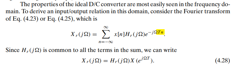
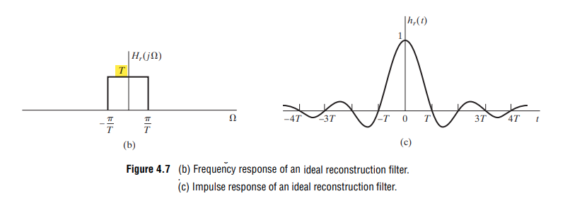
D/C
Zero Padding
Balu Santhanam. ECE-539: Digital Signal Processing: Zero padding and Resolution [http://ece-research.unm.edu/bsanthan/ece539/zero_pad.pdf]
David Castro PiñolDavid Castro Piñol. 𝗭𝗲𝗿𝗼 𝗣𝗮𝗱𝗱𝗶𝗻𝗴 𝗗𝗼𝗲𝘀𝗻’𝘁 𝗜𝗺𝗽𝗿𝗼𝘃𝗲 𝗦𝗽𝗲𝗰𝘁𝗿𝗮𝗹 𝗥𝗲𝘀𝗼𝗹𝘂𝘁𝗶𝗼𝗻 [link]
Zero padding improves frequency grid resolution, not spectral resolution
A smoother spectrum is not more information — it is better interpolation of the same information.
To truly improve spectral resolution, you must observe the signal longer (increase N).
Gotcha
A remarkable fact of linear systems is that the complex exponentials are eigenfunctions of a linear system, as the system output to these inputs equals the input multiplied by a constant factor.
- Both amplitude and phase may change
- but the frequency does not change
For an input \(x(t)\), we can determine the output through the use of the convolution integral, so that with \(x(t) = e^{st}\) \[\begin{align} y(t) &= \int_{-\infty}^{+\infty}h(\tau)x(t-\tau)d\tau \\ &= \int_{-\infty}^{+\infty} h(\tau) e^{s(t-\tau)}d\tau \\ &= e^{st}\int_{-\infty}^{+\infty} h(\tau) e^{-s\tau}d\tau \\ &= e^{st}H(s) \end{align}\]
Take the input signal to be a complex exponential of the form \(x(t)=Ae^{j\phi}e^{j\omega t}\)
\[\begin{align} y(t) &= h(t)*x(t) \\ &= H(j\omega)Ae^{j\phi}e^{j\omega t} \end{align}\]
The frequency response at \(-\omega\) is the complex conjugate of the frequency response at \(+\omega\), given \(h(t)\) is real
\[\begin{align} H^*(t) &= \left(\int_{-\infty}^{+\infty}h(t)e^{-j\omega t}dt\right)^* \\ &= \int_{-\infty}^{+\infty}h^*(t)e^{+j\omega t}dt \\ &= \int_{-\infty}^{+\infty}h(t)e^{-j(-\omega t)}dt \\ &= H(-j\omega) \end{align}\]
The real cosine signal is actually composed of two complex exponential signals: one with positive frequency and the other with negative \[ cos(\omega t + \phi) = \frac{e^{j(\omega t + \phi)} + e^{-j(\omega t + \phi)}}{2} \]
The sinusoidal response is the sum of the complex-exponential response at the positive frequency \(\omega\) and the response at the corresponding negative frequency \(-\omega\) because of LTI systems's superposition property
input: \[\begin{align} x(t) &= A cos(\omega t + \phi) \\ &= \frac{1}{2}Ae^{\phi}e^{\omega t} + \frac{1}{2}Ae^{-\phi}e^{-\omega t} \end{align}\]
output with \(H(j\omega)=Ge^{j\theta}\): \[\begin{align} y(t) &= H(j\omega)\frac{1}{2}Ae^{\phi}e^{\omega t} + H(-j\omega)\frac{1}{2}Ae^{-\phi}e^{-\omega t} \\ &= Ge^{j\theta}\frac{1}{2}Ae^{\phi}e^{\omega t} + Ge^{-j\theta}\frac{1}{2}Ae^{-\phi}e^{-\omega t} \\ &= GAcos(\omega t + \phi + \theta) \end{align}\]
Its phase shift is \(\theta\) and gain is \(G\), which is same with \(H(j\omega)\).
reference
Alan V Oppenheim, Ronald W. Schafer. Discrete-Time Signal Processing, 3rd edition [pdf]
B.P. Lathi, Roger Green. Linear Systems and Signals (The Oxford Series in Electrical and Computer Engineering) 3rd Edition [pdf]
Alan V. Oppenheim, Alan S. Willsky, and S. Hamid Nawab. 1996. Signals & systems (2nd ed.) [pdf]
James H. McClellan, Ronald Schafer, and Mark Yoder. 2015. DSP First (2nd. ed.). Prentice Hall Press, USA