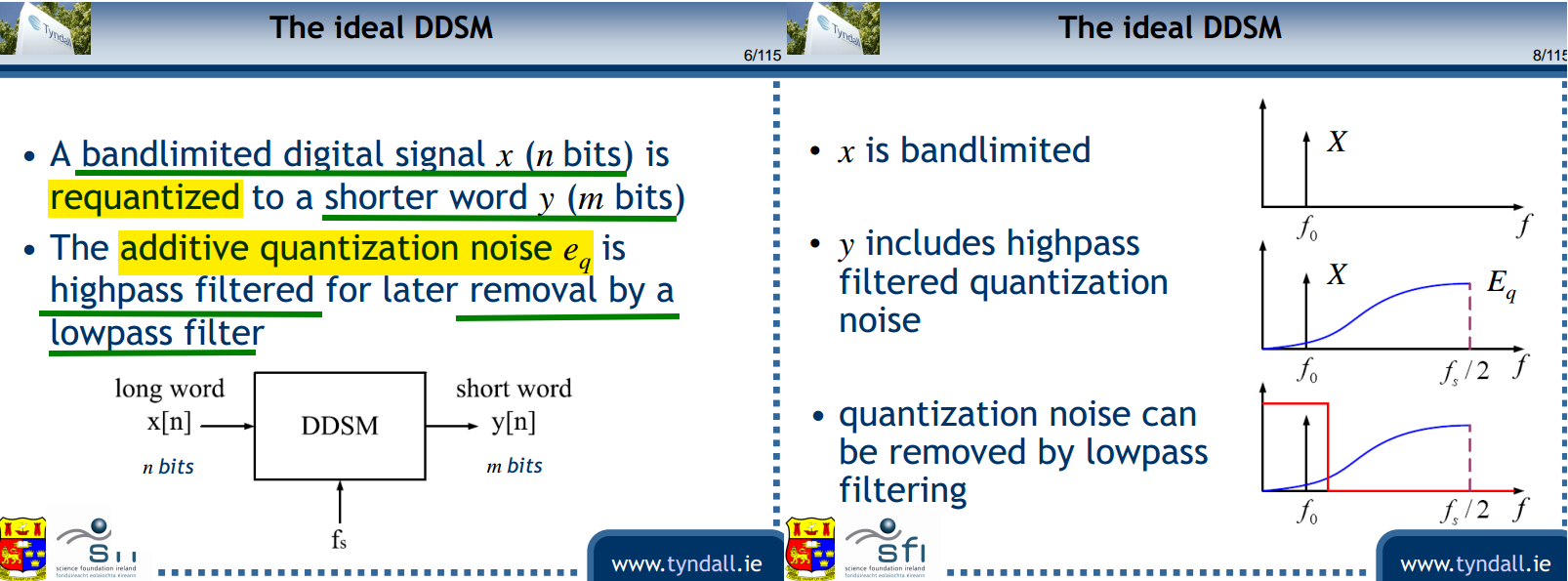
Digital Delta-Sigma Modulators (DDSM)

The DDSM performs integer arithmetic (equivalently, fixed-point with the binary point at the LSB) to realize a fractional value.
linearized model
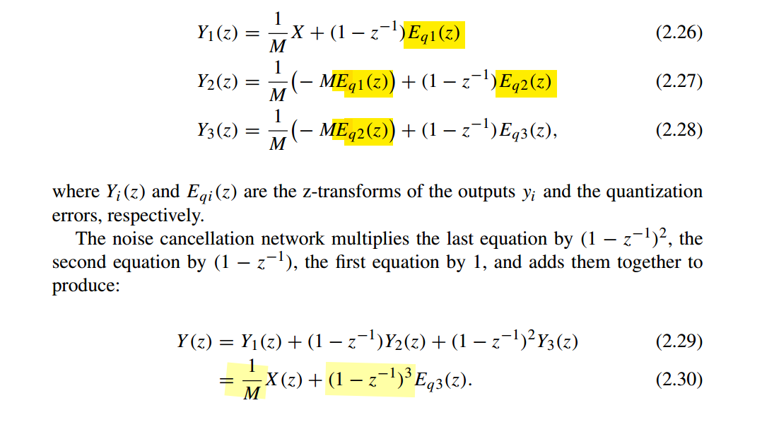
Noise Cancellation Network
 \[\begin{align}
v[n] = \{0,1,2,...,M-1\} &\space\Rightarrow\space y[n] = 0
\space\Rightarrow\space e_q[n] = \{0,
-\frac{1}{M},-\frac{2}{M},...,-\frac{M-1}{M}\} \\
v[n] = \{M,M+1,M2,...,2M-1\} &\space\Rightarrow\space y[n] = 1
\space\Rightarrow\space e_q[n] = \{0,
-\frac{1}{M},-\frac{2}{M},...,-\frac{M-1}{M}\}
\end{align}\]
\[\begin{align}
v[n] = \{0,1,2,...,M-1\} &\space\Rightarrow\space y[n] = 0
\space\Rightarrow\space e_q[n] = \{0,
-\frac{1}{M},-\frac{2}{M},...,-\frac{M-1}{M}\} \\
v[n] = \{M,M+1,M2,...,2M-1\} &\space\Rightarrow\space y[n] = 1
\space\Rightarrow\space e_q[n] = \{0,
-\frac{1}{M},-\frac{2}{M},...,-\frac{M-1}{M}\}
\end{align}\]
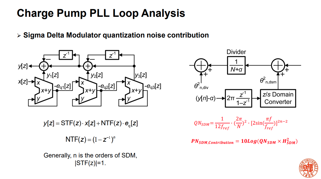
\((1 − z^{−1})^3\)
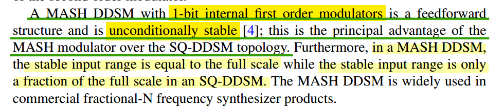
For the three stages of the MASH 1-1-1 DDSM
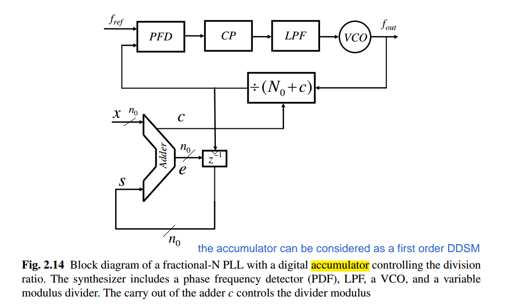
1st order DDSM (digital accumulator)
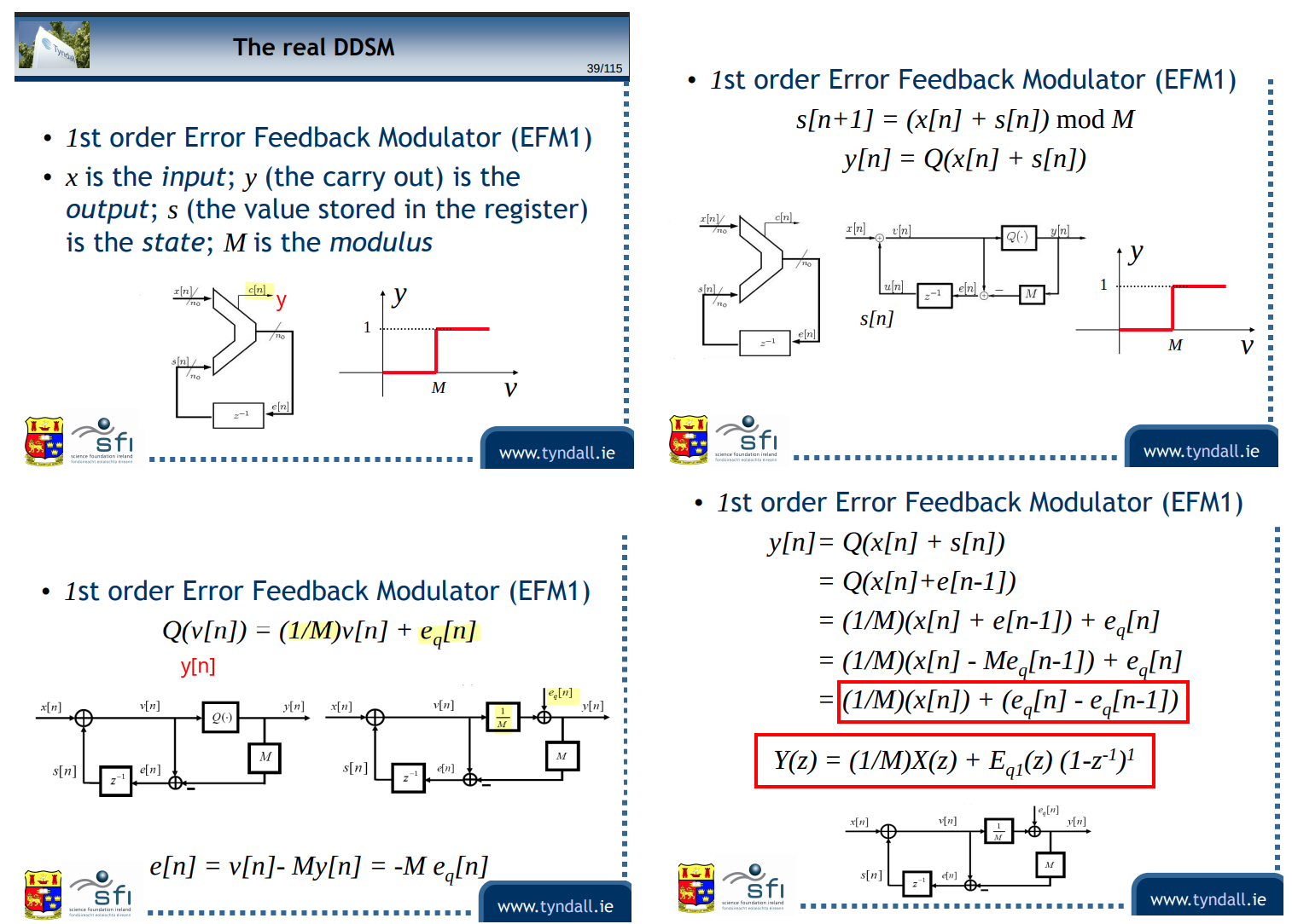
assuming \(n_0=2\)
| \(x[n]+s[n]\) | \(v\) | \(e[n]\) | \(c[n]\), y |
|---|---|---|---|
| 0|00 | 0 | 0 | 0 |
| 0|01 | 1 | 1 | 0 |
| 0|10 | 2 | 2 | 0 |
| 0|11 | 3 | 3 | 0 |
| 1|00 | 4 | 0 | 1 |
| 1|01 | 5 | 1 | 1 |
| 1|10 | 6 | 2 | 1 |
| 1|11 | 7 | 3 | 1 |
yield \(M=2^{n_0}=4\)
2nd order DDSM
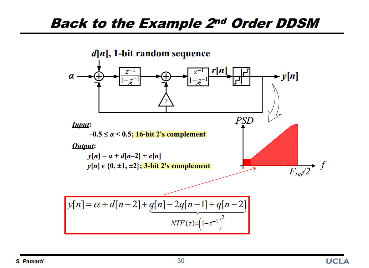
In \(z\)-domain \[ \left\{(A + D - Y)\frac{z^{-1}}{1-z^{-1}} - 2Y \right\}\frac{z^{-1}}{1-z^{-1}} + Q = Y \] That is \[ Y = A z^{-2} + Dz^{-2} + Q(1-z^{-1})^2 \] In time domain \[\begin{align} y[n] &= \alpha[n-2] + d[n-2] + q[n]-2q[n-1]+q[n-2] \\ &= \alpha + d[n-2] + q[n]-2q[n-1]+q[n-2] \end{align}\]
LSB Dither
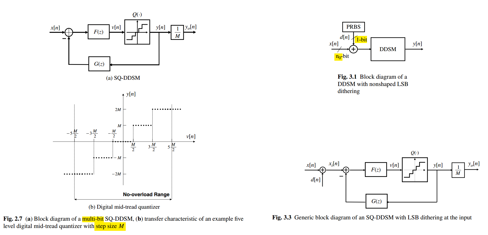
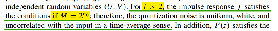
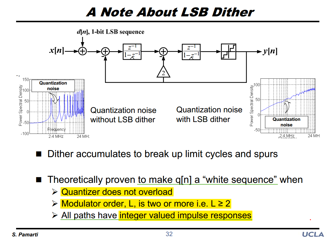
?? integer valued impulse responses
S. Pamarti, J. Welz and I. Galton, "Statistics of the Quantization Noise in 1-Bit Dithered Single-Quantizer Digital Delta–Sigma Modulators," in IEEE Transactions on Circuits and Systems I: Regular Papers, vol. 54, no. 3, pp. 492-503, March 2007 [pdf]
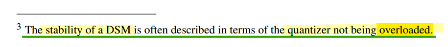
stability of DSM
accumulator wordlength
Z. Ye and M. P. Kennedy, "Hardware Reduction in Digital Delta–Sigma Modulators Via Error Masking—Part II: SQ-DDSM," in IEEE Transactions on Circuits and Systems II: Express Briefs, vol. 56, no. 2, pp. 112-116, Feb. 2009 [https://sci-hub.se/10.1109/TCSII.2008.2010188]
—, "Hardware Reduction in Digital Delta-Sigma Modulators Via Error Masking - Part I: MASH DDSM," in IEEE Transactions on Circuits and Systems I: Regular Papers, vol. 56, no. 4, pp. 714-726, April 2009 [https://sci-hub.se/10.1109/TCSI.2008.2003383]
Truncation DAC
accumulator is implicit quantizer
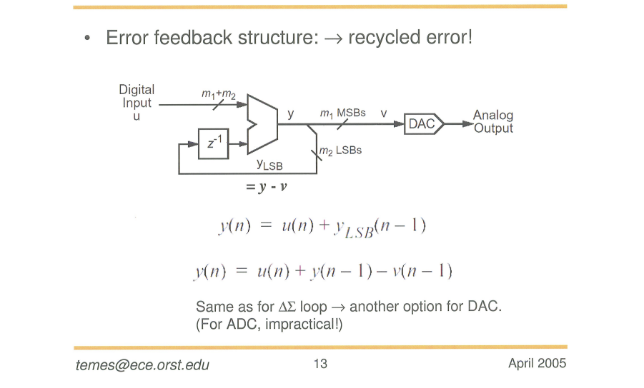
with \(\frac{y}{2^{m_2}} + q= v\), where \(v = \lfloor\frac{y}{2^{m_2}}\rfloor\)
\[ \left\{ \begin{array}{cl} Y + 2^{m_2} Q &= 2^{m_2}V \\ U - z^{-1}2^{m_2}Q &= Y \end{array} \right. \]
The STF & NTF is shown as below \[ V = \frac{1}{2^{m_2}}U + (1-z^{-1})Q \]
To avoid accumulator overflow, stable input range is only of a fraction of the full scale ( \(2^{m_1+m_2}-1\)) \[ u \leq 2^{m_1+m_2} - 2^{m_2} \]
1 | m1 = 2 # MSBs |

To avoid overflow
\[ \log_2(2^k + 2^{N-m}) \leq N \]
Thus \[ N \ge k - \log_2(1 - \frac{1}{2^m}) = k+m -\log_2(2^m-1) \]
suppose \(m\in [1,+\infty)\) \[ k < k - \log_2(1 - \frac{1}{2^m}) \leq k + 1 \] \(N = k +1\) is sufficient for any \(k\)
In the above Temes's sides, \(N = m_1+m_2\) and \(m=m_1\), we have \[ 2^k \leq 2^{m_1+m_2}\cdot (1-\frac{1}{2^{m_1}}) = 2^{m_1+m_2} - 2^{m_2} \]
Generally speaking, \(N \propto k\) and \(N \propto \frac{1}{m}\), especially \(N_{min} = k+1\) if single-bit quantizer \(m=1\)
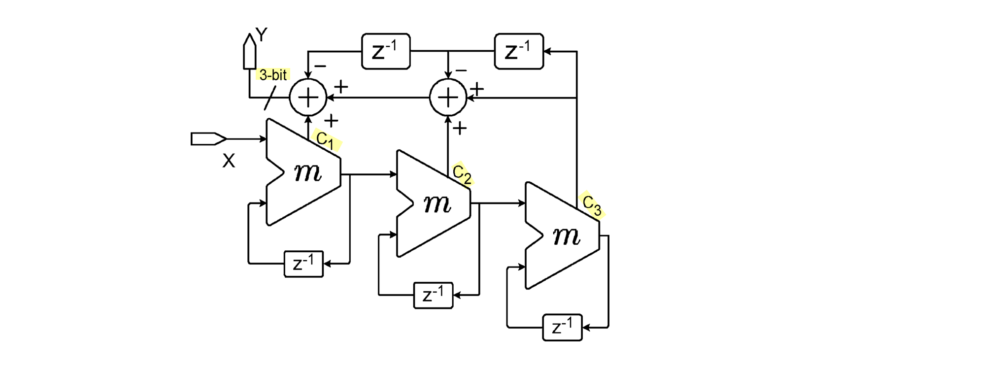
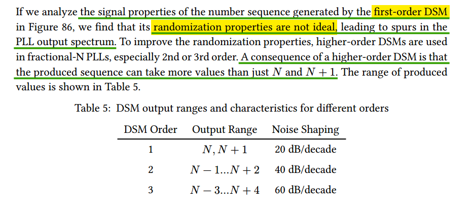
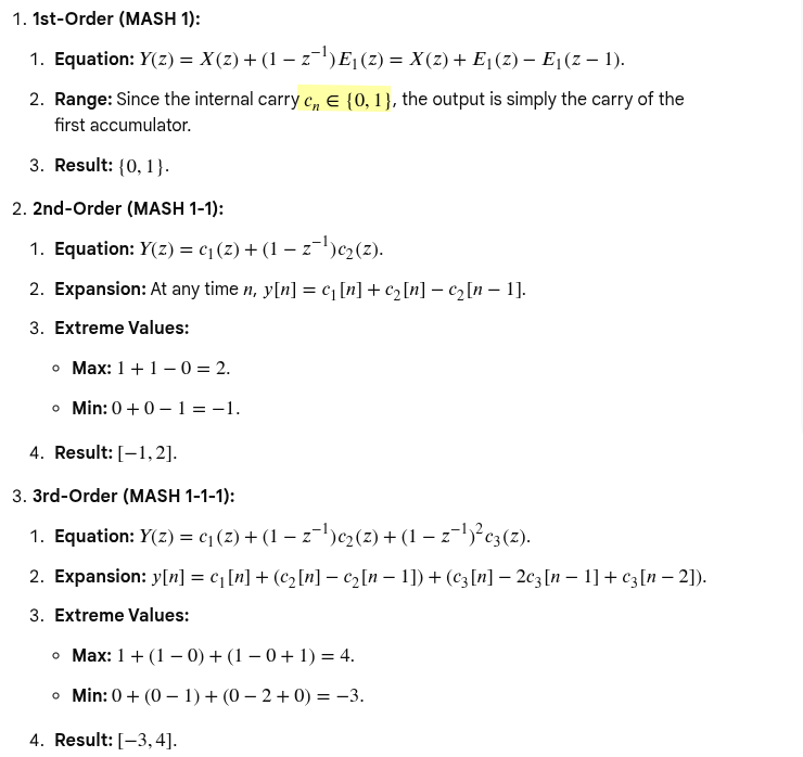
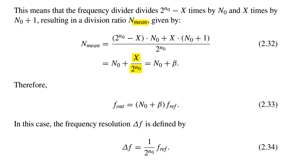
DSM Order & Output Range
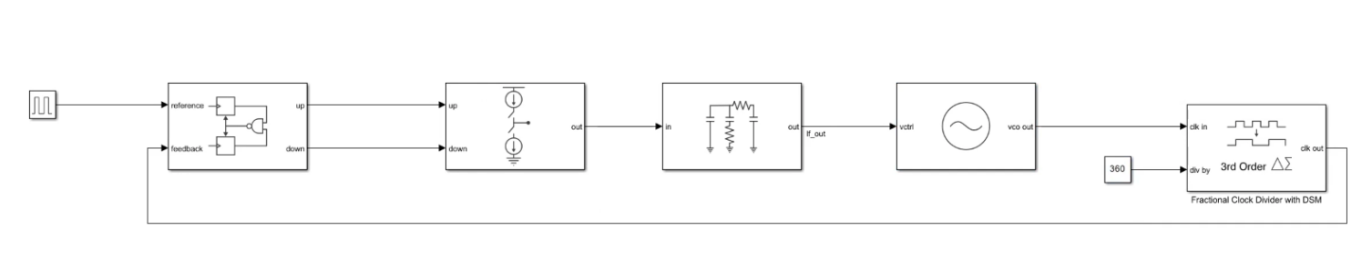
7.4.1 Delta-Sigma Modulator [https://iic-jku.github.io/radio-frequency-integrated-circuits/rfic.html#sec-pll-delta-sigma]
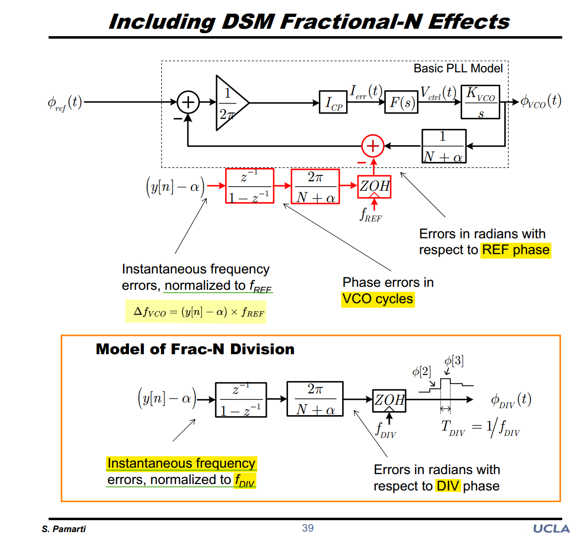
Fractional-N PLL
S. Pamarti, J. Welz and I. Galton, "Statistics of the Quantization Noise in 1-Bit Dithered Single-Quantizer Digital Delta–Sigma Modulators," in IEEE Transactions on Circuits and Systems I: Regular Papers, vol. 54, no. 3, pp. 492-503, March 2007 [https://ispg.ucsd.edu/wordpress/wp-content/uploads/2017/05/2007-TCASI-S.-Pamarti-Statistics-of-the-Quantization-Noise-in-1-Bit-Dithered-Single-Quantizer-Digital-Delta-Sigma-Modulators.pdf]
—. "LSB Dithering in MASH Delta–Sigma D/A Converters," in IEEE Transactions on Circuits and Systems I: Regular Papers, vol. 54, no. 4, pp. 779-790, April 2007 [https://sci-hub.se/10.1109/TCSI.2006.888780]
—. CICC 2020 ES2-2: Basics of Closed- and Open-Loop Fractional Frequency Synthesis [https://youtu.be/t1TY-D95CY8]
Ian Galton. Delta-Sigma Fractional-N Phase-Locked Loops [https://ispg.ucsd.edu/wordpress/wp-content/uploads/2022/10/fnpll_ieee_tutorial_2003_corrected.pdf]
—. ISSCC 2010 SC3: Fractional-N PLLs
—. “Delta-Sigma Fractional-N Phase-Locked Loops.” (2003)
Mike Shuo-Wei Chen, ISSCC 2020 T6: Digital Fractional-N Phase Locked Loop Design
Accumulated Quantization Error (AQE)
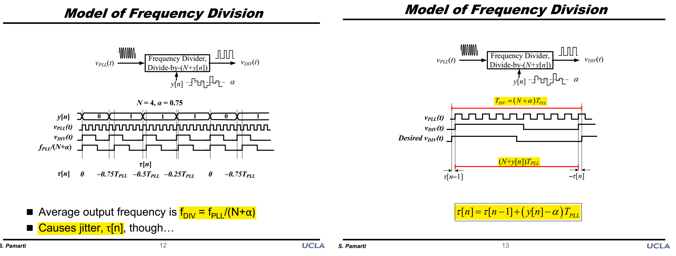 \[
(N+\alpha)T_{PLL} - \tau[n-1] +\tau[n] = (N+y[n])T_{PLL}
\]
\[
(N+\alpha)T_{PLL} - \tau[n-1] +\tau[n] = (N+y[n])T_{PLL}
\]
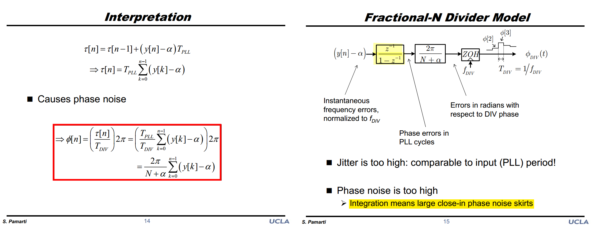
i.e. \[ \tau[n] = \tau[n-1] + (y[n] - \alpha)T_{PLL} \]
where \(\tau[n] = t_{v_{DIV}} - t_{v_{DIV}, desired}\)
Y. Zhang et al., "A Fractional- N PLL With Space–Time Averaging for Quantization Noise Reduction," in IEEE Journal of Solid-State Circuits, vol. 55, no. 3, pp. 602-614, March 2020, [pdf]


X. Wang and M. P. Kennedy, "Unified Analysis of Digital Δ-Σ Modulators (DDSMs) for Fractional-N Frequency Synthesis—Introducing the PASS Family of DDSMs Featuring Independent Shaping of the Probability Density and Spectral Envelope," in IEEE Transactions on Circuits and Systems I: Regular Papers [link]
X. Wang and M. P. Kennedy, "Performance Limits of Fractional-N Digital PLLs with Mid-Rise TDCs," 2023 18th Conference on Ph.D Research in Microelectronics and Electronics (PRIME), Valencia, Spain, 2023 [link]

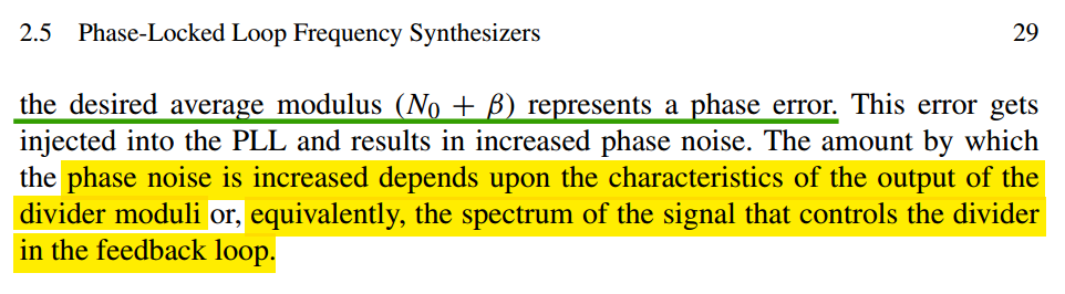
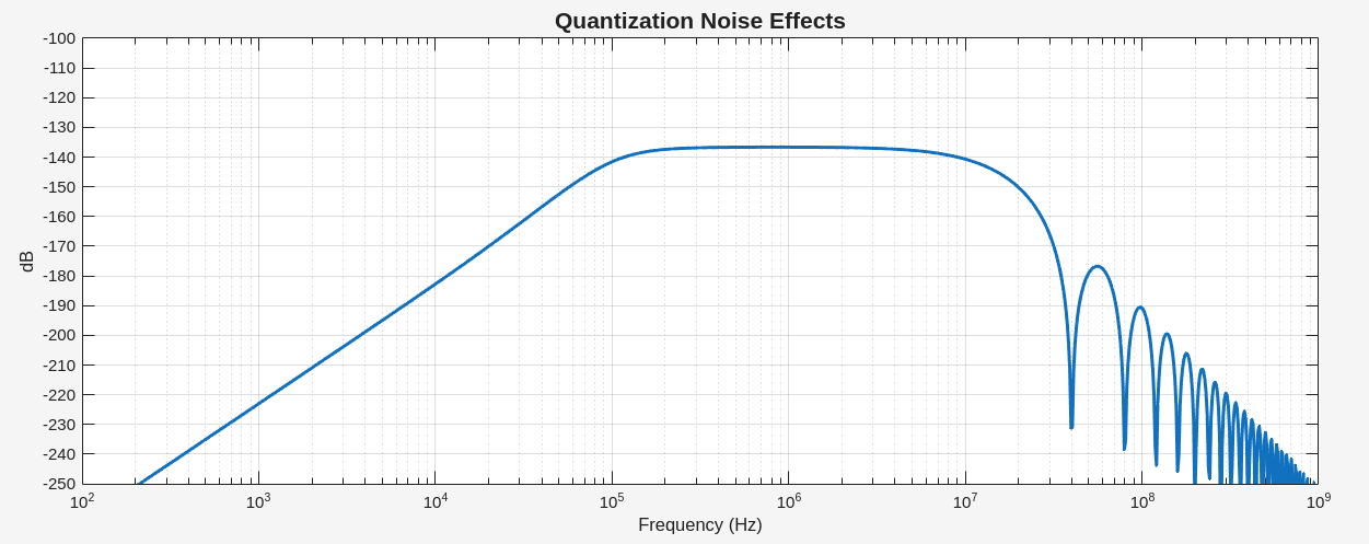
\(\Delta\Sigma\) Noise in PLL
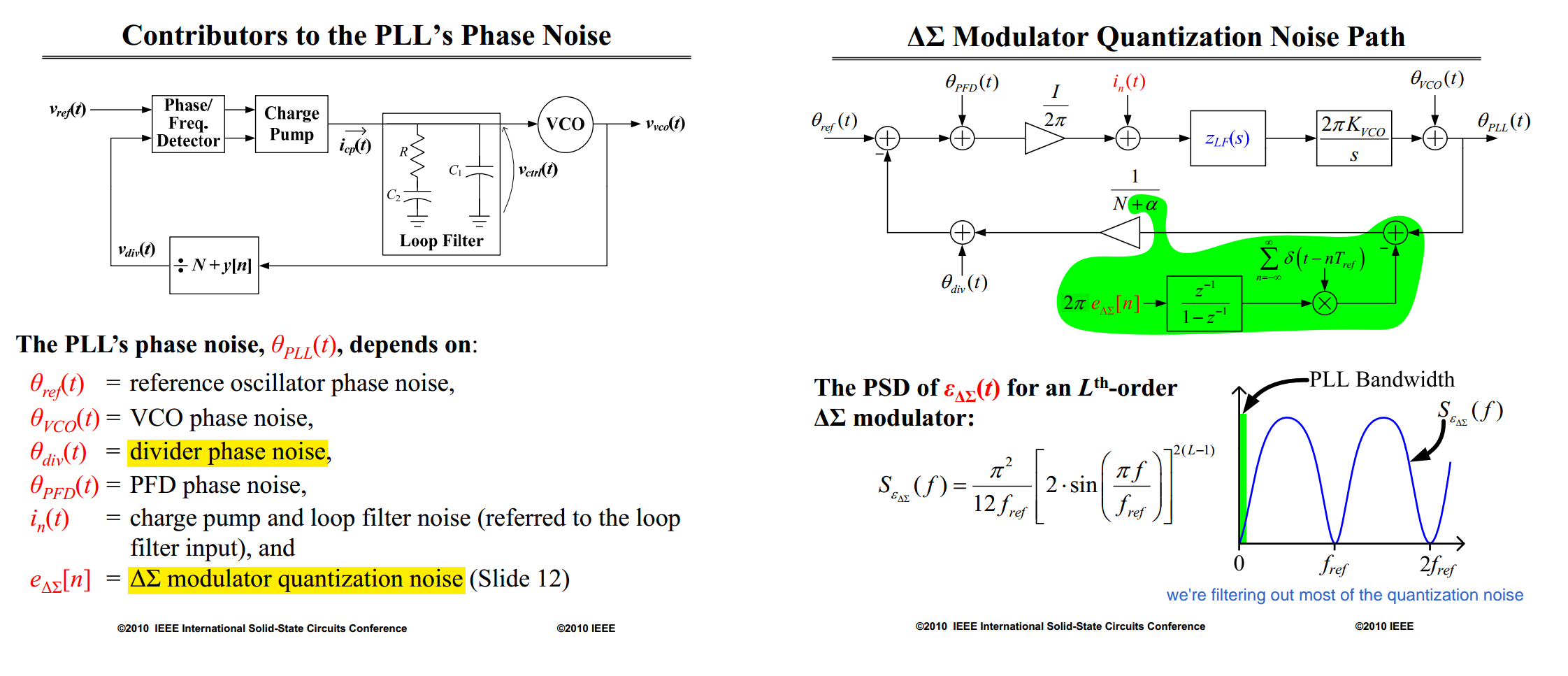
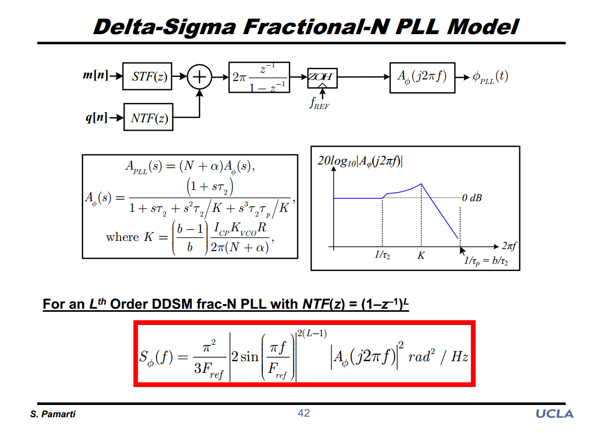

\[\begin{align} S_\phi(f) &= \frac{1}{12F_{ref}}|1-z^{-1}|^{2L}\cdot \left|\frac{2\pi z_{-1}}{1-z^{-1}}\right|^2\cdot \frac{1}{T_{ref}^2} T_{ref}^2 \\ &= \frac{1}{12F_{ref}} |1-z^{-1}|^{2L-2} 4\pi^2 \end{align}\]
with \(|1-z^{-1}| = |2\sin\frac{\pi f}{F_{ref}}|\)
\[ S_\phi(f) = \frac{1}{12F_{ref}} \cdot \left|2\sin\frac{\pi f}{F_{ref}}\right|^{2(L-1)}\cdot 4\pi^2 = \frac{\pi^2}{3F_{ref}} \cdot \left|2\sin\frac{\pi f}{F_{ref}}\right|^{2(L-1)} \]
Jri Lee,【【鳌中堂笔记·抢先体验版】 锁相环08】[bilibili link]
俞思辰, Analog and Digital PLL Phase Noise Model [https://bbs.eetop.cn/thread-996183-1-1.html]
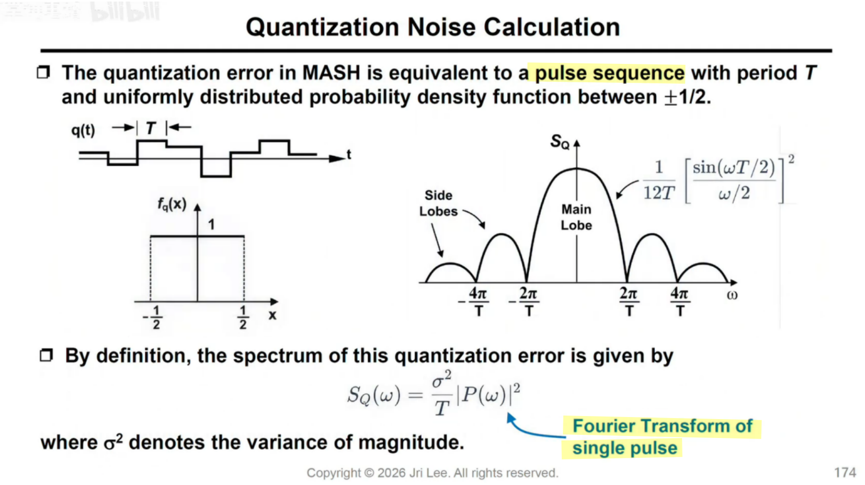
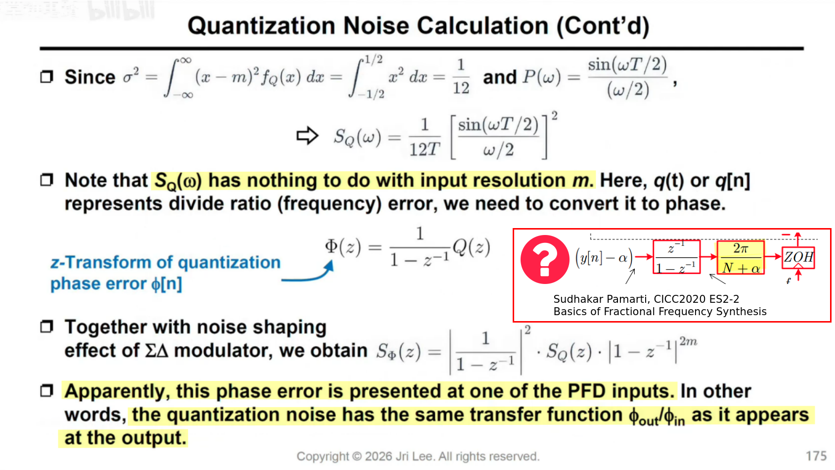
Frequency & Time-Domian Model for Q-noise
metroidman, fractional N量化噪声对系统相位噪声的影响 两种分析方法 LTI频域法和时域采样DFT法 [link]
LTI Frequency domain model & analysis
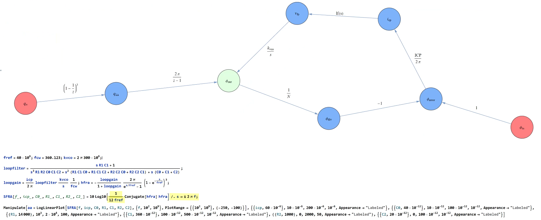
fcw: Frequency Control Word
note
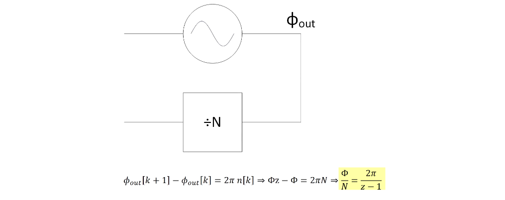
\(z=e^{j2\pi f \color{red}T_\text{ref}}\) — model's time tick is reference clock period
\(\frac{\Phi}{N}(z)\) — relationship between \(\Phi\) and \(N\)
1 | % --- System Parameters --- |
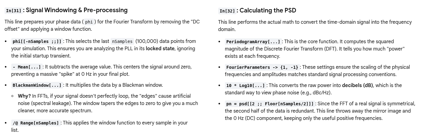
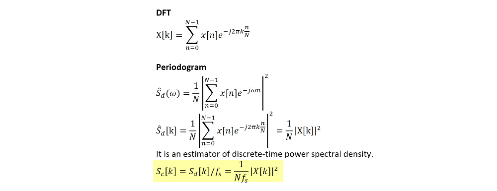
Time domain model & DFT analysis
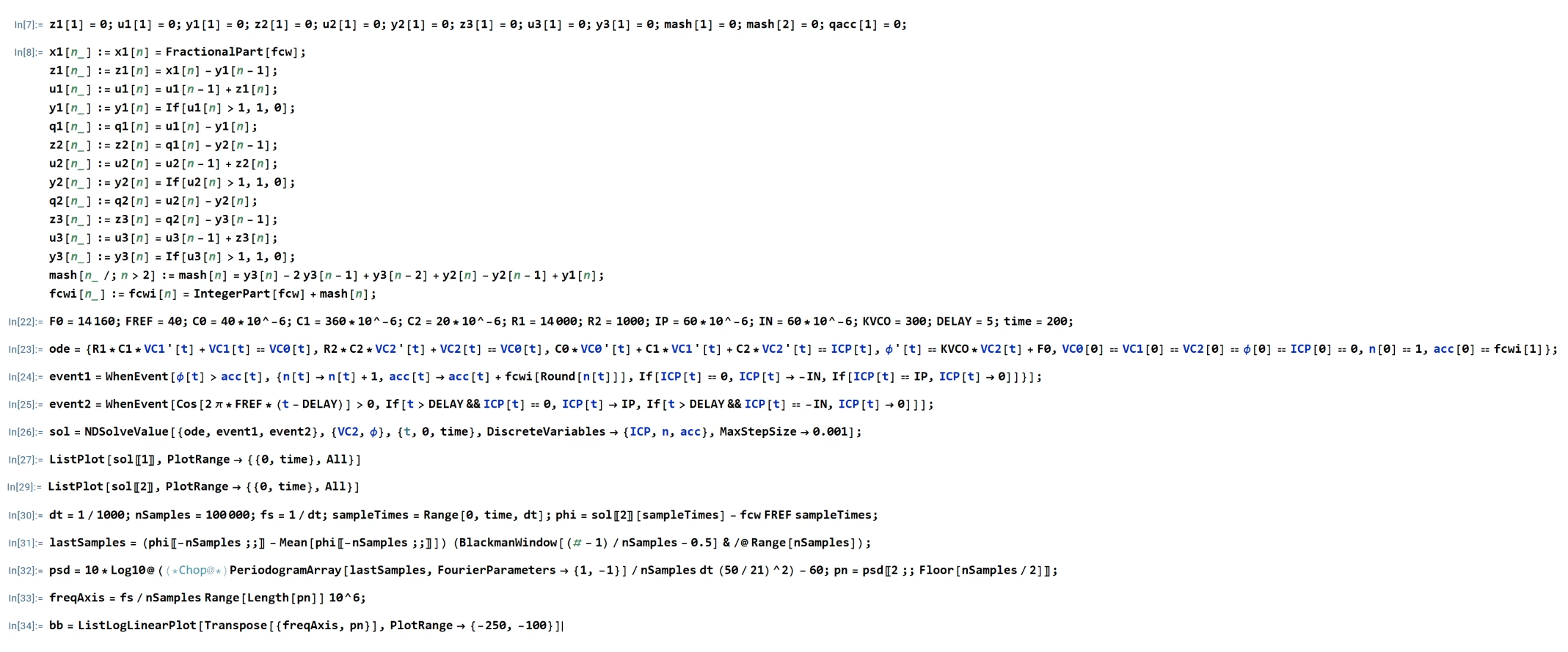
RoundinIn[24]is redundant and likely unnecessary for the logic to function\(\phi\) and
phiis frequency (cycles per second) instead of angular frequency (radians per second)
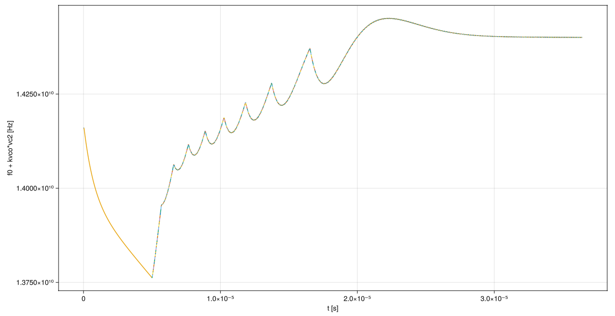
classic PLL module transient response
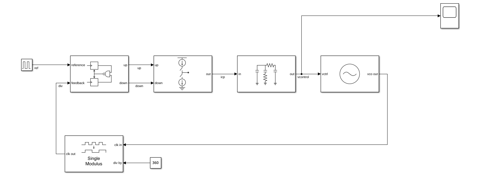
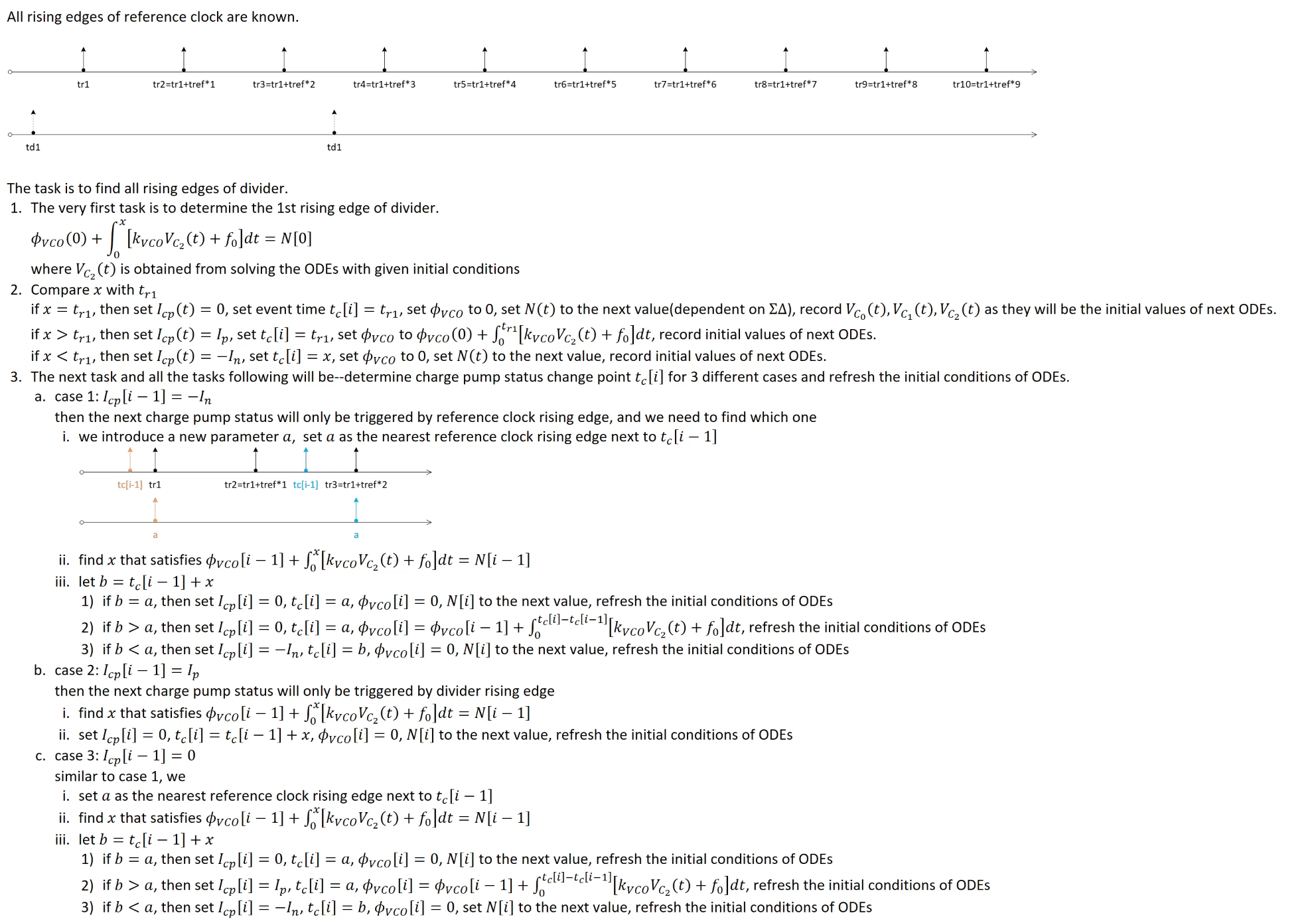
initial state is Reset
classic PLL module in Matlab & Simulink
Kai Wang, Is there a way to improve the code speed? [https://www.mathworks.com/matlabcentral/answers/2039821-is-there-a-way-to-improve-the-code-speed]
classic PLL module in Julia
Julia version (Claude Opus 4.7) [https://gist.github.com/raytroop/53f210b2cca18ec77295dc91dbe35818]
classic PLL module in Mathematica
\(\Delta\Sigma\) DAC
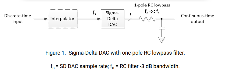
LPF (RC Filter)
Neil Robertson, Model a Sigma-Delta DAC Plus RC Filter [https://www.dsprelated.com/showarticle/1642.php]
Sigma-delta digital-to-analog converters (SD DAC’s) are often used for discrete-time signals with sample rate much higher than their bandwidth
- Because of the high sample rate relative to signal bandwidth, a very simple DAC reconstruction filter (Analog lowpass filter) suffices, often just a one-pole RC lowpass
1 | R= 4.7e3; % ohms resistor value |
1 | % https://www.dsprelated.com/showarticle/1642.php |
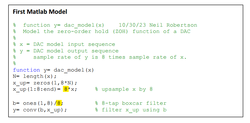
ZOH (Zero-Order Hold Models)
Neil Robertson, DAC Zero-Order Hold Models [https://www.dsprelated.com/showarticle/1627.php]
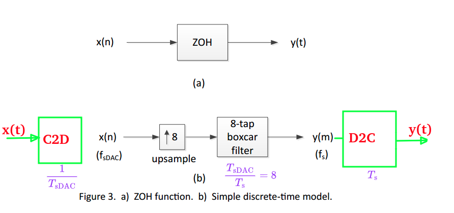
The last D2C is in human vision, which connect discrete time \(y(m)\) with line, implicitly
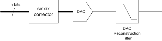
Sinc Corrector
Neil Robertson, Design a DAC sinx/x Corrector [https://www.dsprelated.com/showarticle/1191.php]
Dan Boschen. how to make CIC compensation filter [https://dsp.stackexchange.com/a/31596/59253]
—. Core Building Blocks for Software Defined Radio (SDR): DDC, DUC, NCO) [https://lnkd.in/p/e2MtC9QK]
Equalizing Techniques Flatten DAC Frequency Response [https://www.analog.com/en/resources/technical-articles/equalizing-techniques-flatten-dac-frequency-response.html]
aka. Inverse Sinc Compensation
TODO 📅
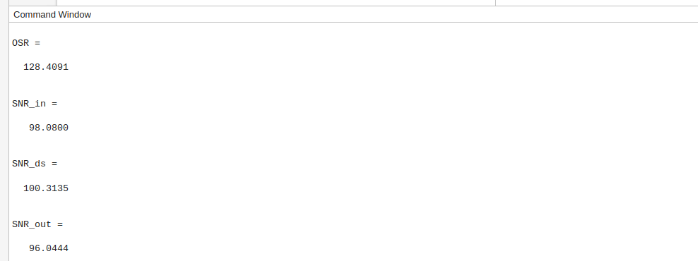
OSR & NS
maximum output signal 22kHz
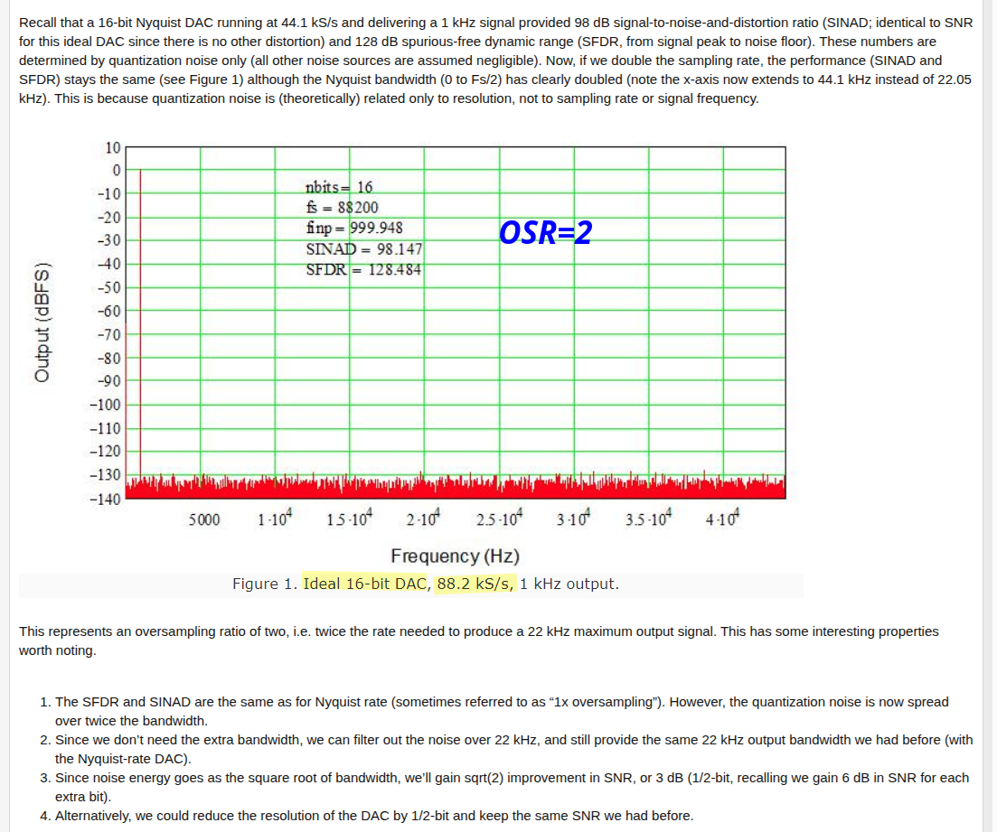
\[SNR = 16\times 6.02 + 1.76 = 98.08\]
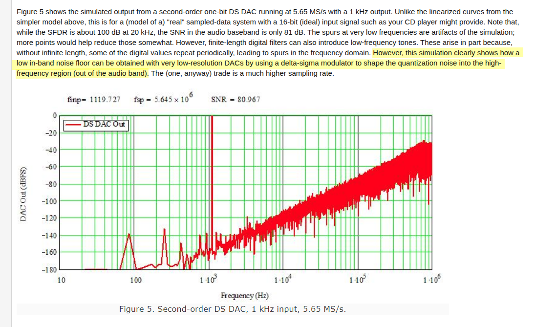
1 | OSR = 5.65e6/(2*22e3); |
Y. Liu, J. Gao and X. Yang, "24-bit low-power low-cost digital audio sigma-delta DAC," in Tsinghua Science and Technology, vol. 16, no. 1, pp. 74-82, Feb. 2011 [https://ieeexplore.ieee.org/stamp/stamp.jsp?arnumber=6077939]
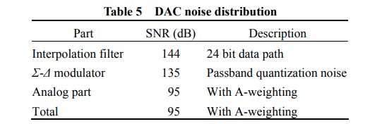
1 | snr_if = 144; |
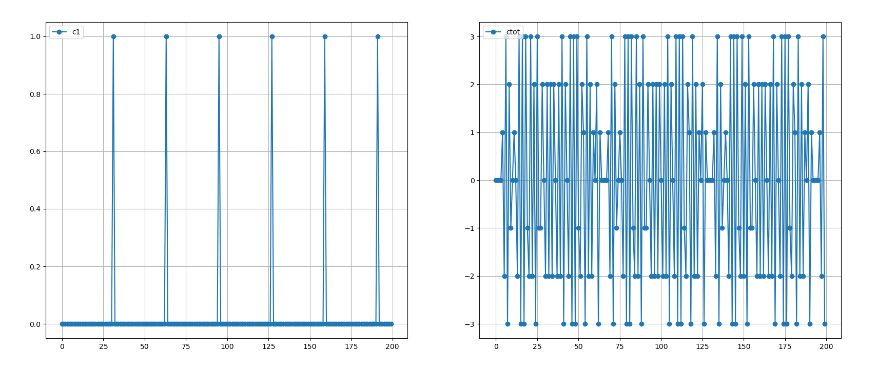
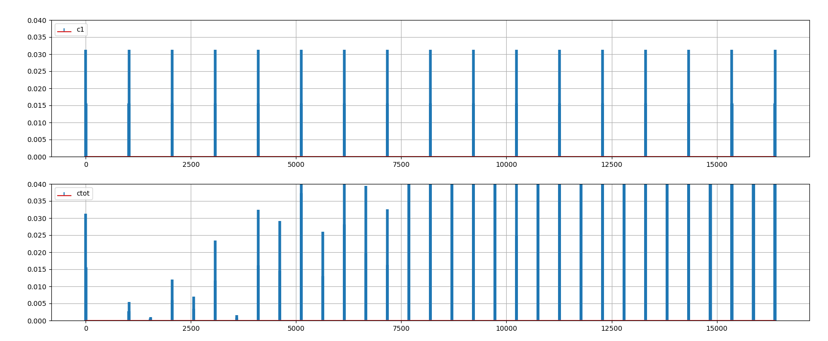
MASH 1-1-1 Model
J. W. M. Rogers, F. F. Dai, M. S. Cavin and D. G. Rahn, "A multiband /spl Delta//spl Sigma/ fractional-N frequency synthesizer for a MIMO WLAN transceiver RFIC," in IEEE Journal of Solid-State Circuits, vol. 40, no. 3, pp. 678-689, March 2005 [https://sci-hub.se/10.1109/JSSC.2005.843604]
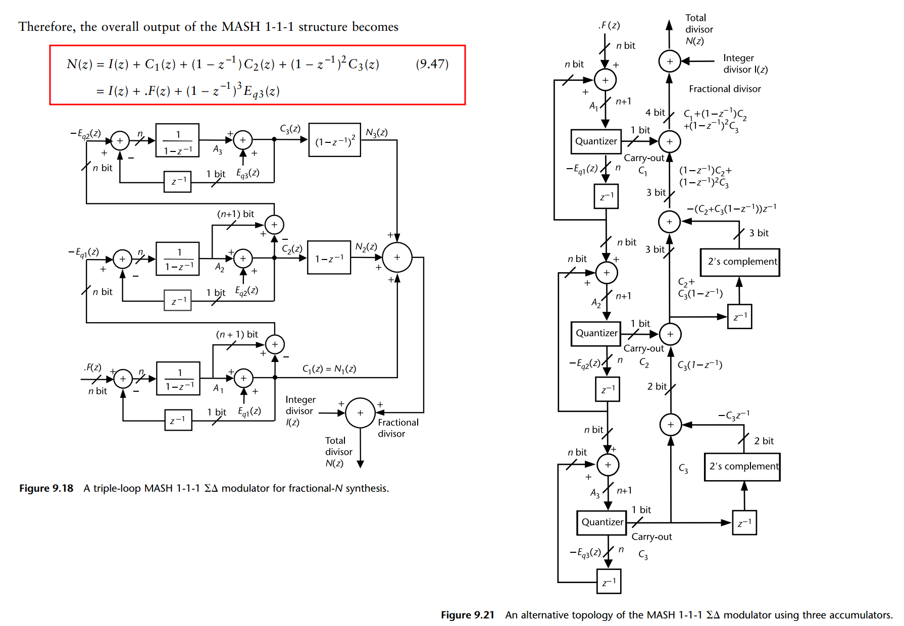
(a) a fractional accumulator, and (b) a triple-loop \(\Delta\Sigma\) accumulator for \(N(z) = 100 + 1/32\)
\(n=5\)
1 | import numpy as np |
Harald Pretl, Radio-Frequency Integrated Circuits. 7.4 Fractional-N PLL [note] [MASH Modulator (3rd Order) code]

1 | # Stage 1: 1st order modulator with input signal |
1 | for i in range(length): |
1 | # Plot 2: Frequency spectrum (with dither) |

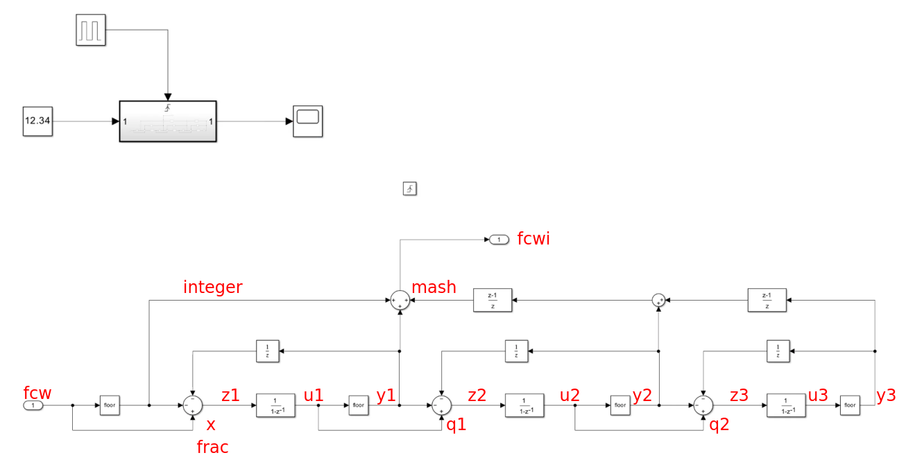
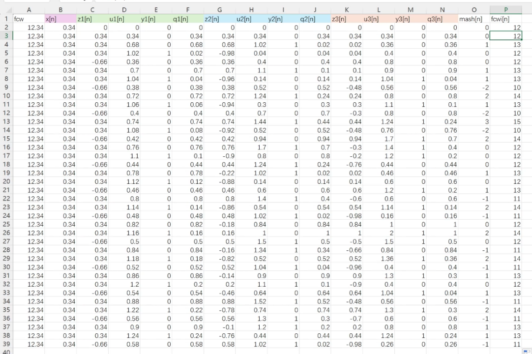
metroidman, 用Simulink Excel Mathematica三种不同工具从零搭建3阶ΣΔ调制器并进行时域和频率分析 [link]
Simulink
Excel
Mathematica
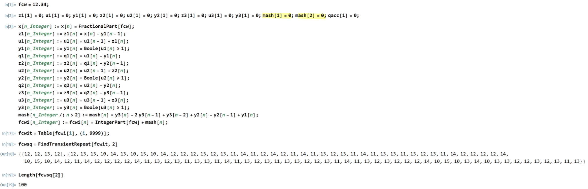
The code fcwit = Table[fcwi[i], {i, 9999}]; is the
command that actually runs the simulation for a set
duration.
Here is the breakdown of what is happening:
Table[..., {i, 9999}]: This creates a list by repeating an operation 9,999 times. It acts like aforloop in other programming languages.fcwi[i]: This calls the function you defined earlier. For every value ofifrom 1 to 9,999, it calculates the instantaneous integer division ratio produced by the MASH modulator.fcwit = ...: It stores all 9,999 results into a single long list (an array) namedfcwit.;(Semicolon): This is important—it suppresses the output. Without it, Mathematica would print all 9,999 numbers on your screen, which would be a huge mess!
reference
Michael Peter Kennedy. scv-cas 2014: Digital Delta-Sigma Modulators [pdf,recording]
—, Recent advances in the analysis, design and optimization of Digital Delta-Sigma Modulators [pdf]
Kaveh Hosseini and Peter Kennedy. 2006 Hardware Efficient Maximum Sequence Length Digital MASH Delta Sigma Modulator [pdf]
Jason Sachs. Return of the Delta-Sigma Modulators, Part 1: Modulation [https://www.dsprelated.com/showarticle/1517/return-of-the-delta-sigma-modulators-part-1-modulation]
Neil Robertson, Modeling a Continuous-Time System with Matlab [https://www.dsprelated.com/showarticle/1055.php]
—, “A Simplified Matlab Function for Power Spectral Density”, DSPRelated.com, March, 2020, [https://www.dsprelated.com/showarticle/1333.php]
Rick Lyons. How Discrete Signal Interpolation Improves D/A Conversion [https://www.dsprelated.com/showarticle/167.php]
Dan Boschen. sigma delta modulator for DAC [https://dsp.stackexchange.com/a/88357/59253]
Woogeun Rhee. ISCAS 2019 Mini Tutorials: Single-Bit Delta-Sigma Modulation Techniques for Robust Wireless Systems [https://youtu.be/OEyTM4-_OyA]
—, 2001 Phd Thesis: Multi-Bit Delta -Sigma Modulation Technique for Fractional-N Frequency Synthesizers [https://www.ime.tsinghua.edu.cn/Thesis_rhee.pdf]
Pavan, Shanthi, Richard Schreier, and Gabor Temes. (2016) 2016. Understanding Delta-Sigma Data Converters. 2nd ed. Wiley.
John Rogers, Calvin Plett, and Foster Dai. 2006. Integrated Circuit Design for High-Speed Frequency Synthesis (Artech House Microwave Library). Artech House, Inc., USA.
K. Hosseini and M. P. Kennedy, Minimizing Spurious Tones in Digital Delta-Sigma Modulators (Analog Circuits and Signal Processing). New York, NY, USA: Springer, 2011.
Rhee, W. (2020). Phase-locked frequency generation and clocking : architectures and circuits for modern wireless and wireline systems. The Institution of Engineering and Technology
Lacaita, Andrea Leonardo, Salvatore Levantino, and Carlo Samori. Integrated frequency synthesizers for wireless systems. Cambridge University Press, 2007.