Multirate Filter
alternative view of sampling, assuming DC value is \(A\)
\(x_c(t)\) and \(x_s(t)\)
\(\overline{x_c} = A\); \(\overline{x_s}=\frac{A}{T}\): therefore \(X_s(j0) = \frac{1}{T}X_c(j0)\)
\(x[n]\) and \(x_d[n]\)
\(\overline{x} = A\); \(\overline{x_d}=\frac{A}{2}\): therefore \(X_d(e^{j0}) = \frac{1}{2}X(e^{j0})\)
expander
\(x[n]\) and \(x_e[n]\)
\(\overline{x} = A\); \(\overline{x_e}=A\): therefore \(X_e(e^{j0}) = X(e^{j0})\)
Fourier transform of the output of the expander is a frequency-scaled version of the Fourier transform of the input
Subsampling or Downsampling

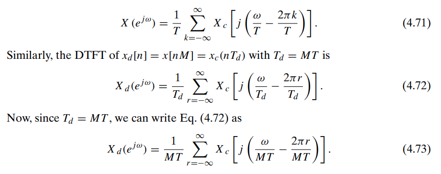
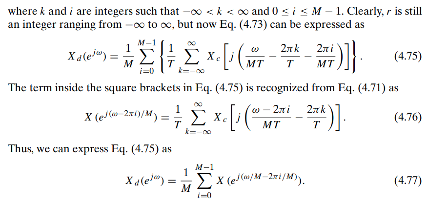
Eqs. (4.72)
the superposition of an infinite set of amplitude-scaled copies of \(X_c(j\Omega)\), frequency scaled through \(\omega = \Omega T_d\) and shifted by integer multiples of \(2\pi\)
Eq. (4.77)
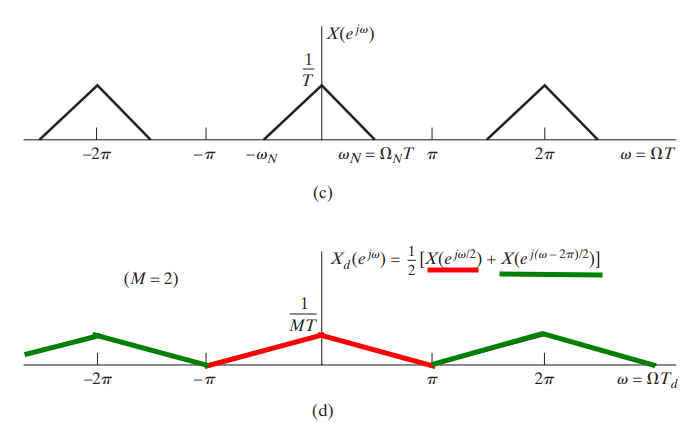
the superposition of \(M\) amplitude-scaled copies of the periodic Fourier transform \(X (e^{j\omega})\), frequency scaled by \(M\) and shifted by integer multiples of \(2\pi\)
downsampled by a factor of \(M = 2\)


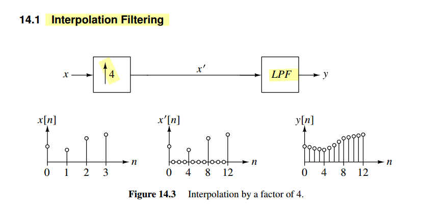
Upsampling or Zero Insertion


Rouphael, Tony. (2009). RF and Digital Signal Processing for Software-Defined Radio. [pdf]
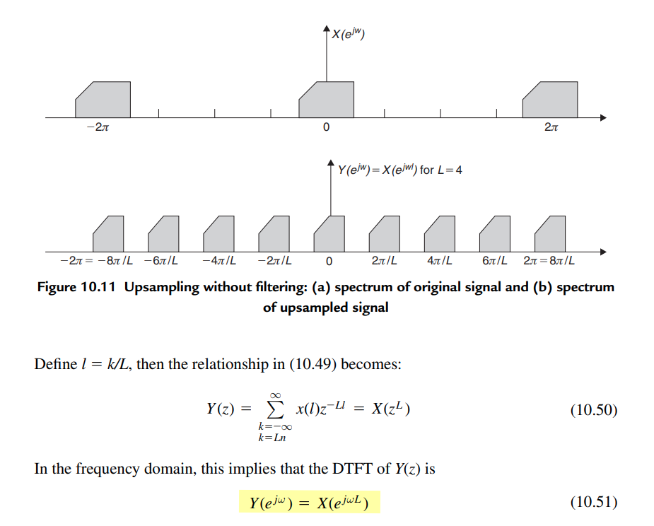

Assuming \(X(e^{j\omega_1}) = U_f(e^{j\omega_1})\) with \(\omega_1 = \Omega T_1\), upsampled by ratio \(L\), then obtain
\[ Y(e^{j\omega_2})=X(e^{j\omega_2 L}) = U_f(e^{j\omega_2 L}) \]
by EQ. (4.85), i.e. substitute \(\omega_1\) with \(\omega_2 L\), where with \(\omega_2 = \Omega T_2\) and \(T_2 L = T_1\)
Provided that \(\xi = e^{j\omega_1}\) and \(z = e^{j\omega_2}\), we have \(U_f(\xi)\) upsampled to \(U_f(z^L)\)
Interpolation filter
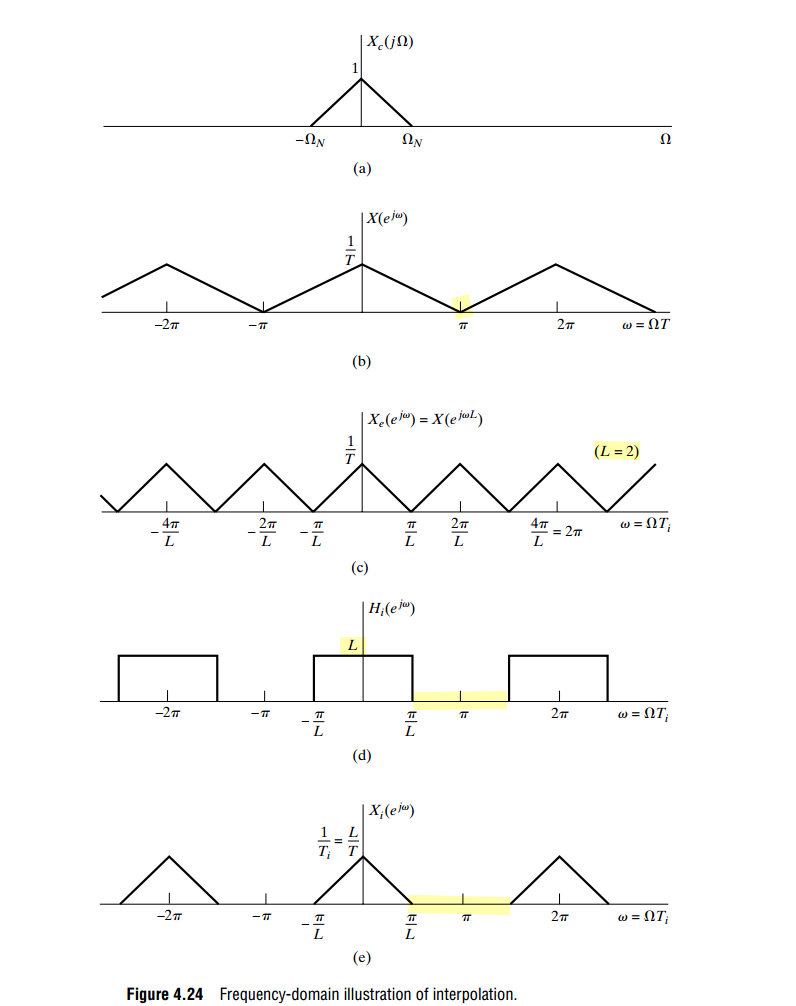
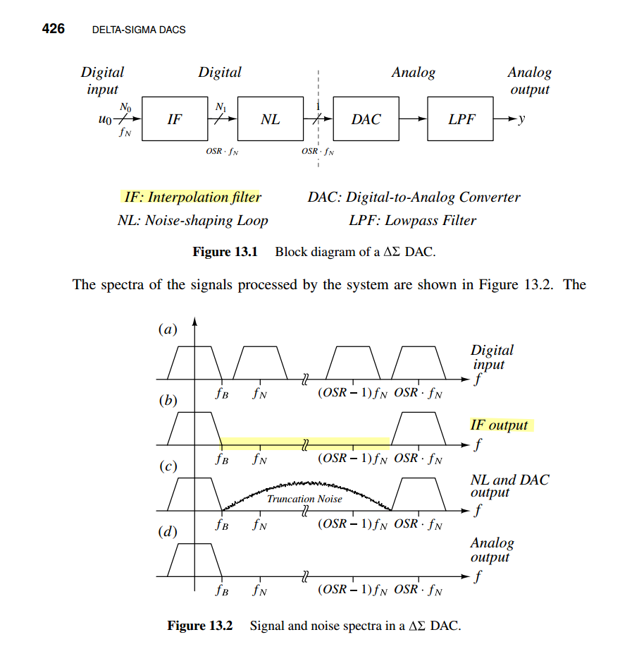
Pavan, Schreier and Temes, "Understanding Delta-Sigma Data Converters, Second Edition"
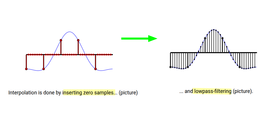
Markus Nentwig. Polyphase filter / Farrows interpolation [https://www.dsprelated.com/showarticle/22.php]
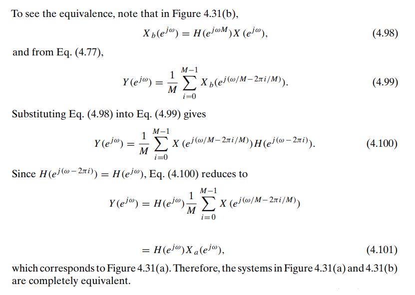
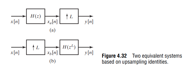
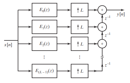
sampling identities
downsampling identity
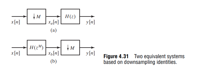
upsampling identity
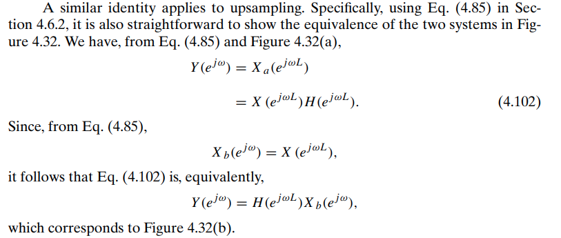
Polyphase Decomposition
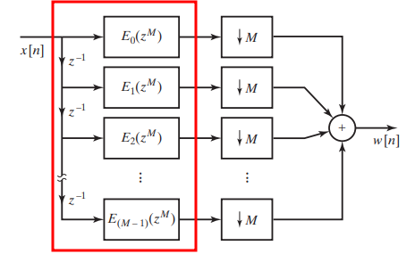
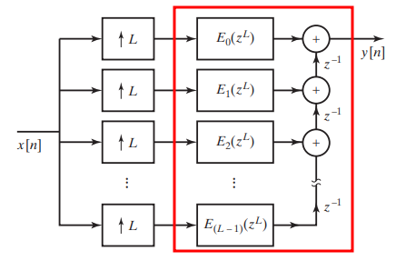
Polyphase decomposition is a powerful technique used in digital signal processing to efficiently implement multirate systems.
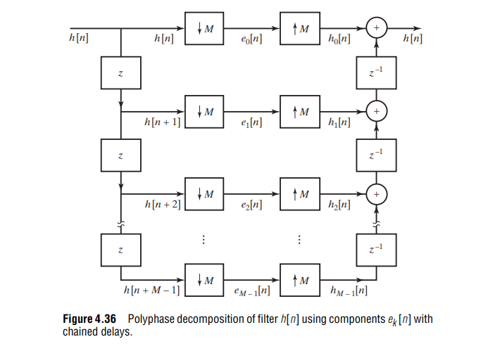

where \(e_k[n]=h[nM+k]\)
Polyphase Implementation of Decimation Filters & Interpolation Filters
| Decimation system | Interpolation system | |
|---|---|---|
 |
 |
|
 |
 |
|
| sampling identity | 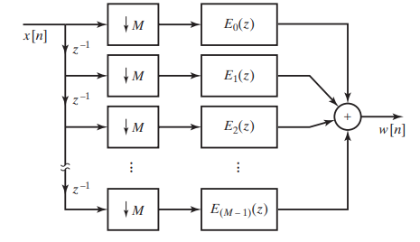 |
 |
LPTV Implementation
TODO 📅
The interpolation filter following an up-sampler generally is time varying and cannot be represented by a simple transfer function. The equivalent filter in a zero-order hold is an exception, perhaps unique, that can be represented with a time-invariant transfer function
Dr. Deepa Kundur, Multirate Digital Signal Processing: Part I [pdf, https://www.comm.utoronto.ca/dkundur/course/discrete-time-systems/]
ZOH interpolator
The interpolation filter following an up-sampler generally is time varying and cannot be represented by a simple transfer function. The equivalent filter in a Zero-Order Hold is an exception, perhaps unique, that can be represented with a time-invariant transfer function
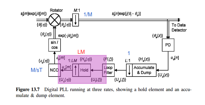
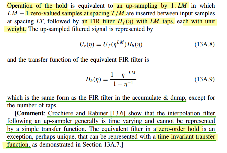
\[
F_1(z) = X(z^{LM})\frac{1-z^{-LM}}{1-z^{-1}}
\]
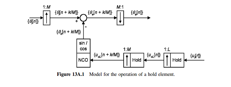
Split the \(1:LM\) hold process into a \(1 : L\) hold followed by a \(1 : M\) hold \[ Y(\eta)=X(\eta^{L})\frac{1-\eta^{-L}}{1-\eta^{-1}} \] then \[\begin{align} F_2(z) &= Y(z^M)\cdot\frac{1-z^{-M}}{1-z^{-1}} \\ &=X(z^{LM})\frac{1-z^{-LM}}{1-z^{-M}}\cdot \frac{1-z^{-M}}{1-z^{-1}} \\ &= X(z^{LM})\frac{1-z^{-LM}}{1-z^{-1}} \end{align}\]
That is \(F_1(z)=F_2(z)\), i.e. they are equivalent
Random Signals & Multirate Systems
Balu Santhanam, Probability Theory & Stochastic Process 2020: Random Signals & Multirate Systems [https://ece-research.unm.edu/bsanthan/ece541/rand.pdf]
Decimation by Summing
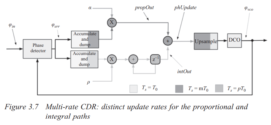
proportional path
The loop gain of a proportional path is unchanged
In (a), the loop gain is \(\frac{\phi_o(z)}{\phi_e(z)}\), which is \[ LG_a(z)=\frac{\phi_o(z)}{\phi_e(z)} = \frac{1}{1-z^{-1}} \]
In (b), Accumulate-And-Dump (AAD) is \(\frac{1-z^{-L}}{1-z^{-1}}\), then \(\phi_m(\eta)\) can be expressed as \[ \phi_m(\eta) = \frac{1-\eta^{-1}}{1-\eta^{-1/L}}\cdot \frac{1}{L} \] Hence \[\begin{align} \phi_o(\eta) &= \phi_m(\eta) \frac{1}{1-\eta^{-1}} \\ &= \frac{1-\eta^{-1}}{1-\eta^{-1/L}}\cdot \frac{1}{L}\cdot \frac{1}{1-\eta^{-1}} \end{align}\]
After zero-order hold process, we obtain \(\phi_f(z)\), which is \[\begin{align} \phi_f(z) &= \phi_o(z^L) \cdot \frac{1-z^{-L}}{1-z^{-1}} \\ &=\frac{1-z^{-L}}{1-z^{-1}}\cdot \frac{1}{L}\cdot \frac{1}{1-z^{-L}}\cdot \frac{1-z^{-L}}{1-z^{-1}} \end{align}\] i.e., \[ LG_b(z) = \frac{1}{1-z^{-1}}\cdot \frac{1}{L}\cdot \frac{1-z^{-L}}{1-z^{-1}} \]
When bandwidth is much less than sampling rate (data rate), \(\frac{1}{L}\cdot \frac{1-z^{-L}}{1-z^{-1}} \approx 1\)
Therefore \[ LG_b(z) \approx \frac{1}{1-z^{-1}} \]
In the end \[ LG_a(z) \approx LG_b(z) \]
Assume PD output is constant
integral path
integral path gain reduced by \(L\)
In (a), \(\phi_o(z)=\frac{1}{(1-z^{-1})^2}\), i.e. \[ LG_a(z) = \frac{1}{(1-z^{-1})^2} \]
In (b), after Accumulate-And-Dump (AAD), \(\phi(\eta)\) is \[ \phi_m(\eta) = \frac{1-\eta^{-1}}{1-\eta^{-1/L}}\cdot \frac{1}{L} \]
After frequency integrator and phase integrator \[\begin{align} \phi_o(\eta) &= \phi_m(\eta) \cdot \frac{1}{(1-\eta^{-1})^2} \\ &= \frac{1-\eta^{-1}}{1-\eta^{-1/L}}\cdot \frac{1}{L} \cdot \frac{1}{(1-\eta^{-1})^2} \end{align}\] Then \(\phi_f(z)\) is shown as below \[\begin{align} \phi_f(z) &= \phi_o(z^L)\cdot \frac{1-z^{-L}}{1-z^{-1}} \\ &= \frac{1-z^{-L}}{1-z^{-1}}\cdot \frac{1}{L}\cdot \frac{1}{(1-z^{-L})^2}\cdot \frac{1-z^{-L}}{1-z^{-1}} \\ &= \frac{1}{L} \cdot \frac{1}{(1-z^{-1})^2} \end{align}\]
That is, \[ LG_b(z) = \frac{1}{L} \cdot \frac{1}{(1-z^{-1})^2} = \frac{1}{L}\cdot LG_a(z) \]
Assume PD output is constant
\[ \lim_{n\to +\infty} \frac{\Delta P_1}{\Delta P_0} = \lim_{n\to +\infty}\frac{n+2L}{nL+\alpha L+\beta L^2} = \frac{1}{L} \]
Decimation by Voting
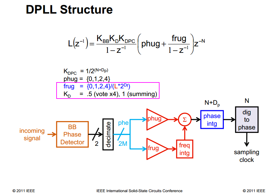
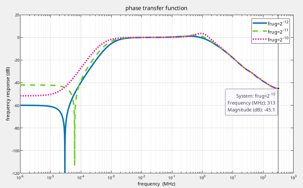
In above screenshot
- \(K_D\) is just relative value
- frug shall not be scaled by decimator factor
proved as below
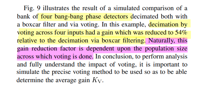
DC gain \(K_B\) of summing (boxcar filter) is decimation factor \(M\) , voting gain \(K_V\) is about \(0.54K_b=0.54M\)
- downsampling \(\frac{1}{M}\) and ZOH \(\frac{1-z^{-M}}{1-z^{-1}}\) can be canceled out at low frequency
- decimation gain: accumulator \(\frac{1-z^{-M}}{1-z^{-1}}\) replaced with linearizing gain \(K_B\) and majority voting replaced with \(K_V\)
proportional path: \[\begin{align} LG_{ph} &= K_{BB}\cdot \frac{1-z^{-M}}{1-z^{-1}}\cdot \frac{1}{M}\cdot \frac{1}{1-z^{-M}}\cdot \frac{1-z^{-M}}{1-z^{-1}} \\ &\approx K_{BB}\cdot \frac{1-z^{-M}}{1-z^{-1}}\cdot \frac{1}{1-z^{-M}} \\ &= K_{BB}\cdot K_D\cdot \frac{1}{1-z^{-M}} \end{align}\]
integral path: \[\begin{align} LG_{fr} &= K_{BB}\cdot \frac{1-z^{-M}}{1-z^{-1}}\cdot \frac{1}{M}\cdot \frac{1}{(1-z^{-M})^2}\cdot \frac{1-z^{-M}}{1-z^{-1}} \\ &\approx K_{BB}\cdot \frac{1-z^{-M}}{1-z^{-1}}\cdot \frac{1}{(1-z^{-M})^2} \\ &= K_{BB}\cdot K_D\cdot \frac{1}{(1-z^{-M})^2} \end{align}\]
J. Stonick. ISSCC 2011 "DPLL-Based Clock and Data Recovery" [slides,transcript]
J. L. Sonntag and J. Stonick, "A Digital Clock and Data Recovery Architecture for Multi-Gigabit/s Binary Links," in IEEE Journal of Solid-State Circuits, vol. 41, no. 8, pp. 1867-1875, Aug. 2006 [https://sci-hub.se/10.1109/JSSC.2006.875292]
J. Sonntag and J. Stonick, "A digital clock and data recovery architecture for multi-gigabit/s binary links," Proceedings of the IEEE 2005 Custom Integrated Circuits Conference, 2005.. [https://sci-hub.se/10.1109/CICC.2005.1568725]
Y. Xia et al., "A 10-GHz Low-Power Serial Digital Majority Voter Based on Moving Accumulative Sign Filter in a PS-/PI-Based CDR," in IEEE Transactions on Microwave Theory and Techniques, vol. 68, no. 12 [https://sci-hub.se/10.1109/TMTT.2020.3029188]
J. Liang, A. Sheikholeslami, "On-Chip Jitter Measurement and Mitigation Techniques for Clock and Data Recovery Circuits" [https://tspace.library.utoronto.ca/bitstream/1807/91138/3/Liang_Joshua_201706_PhD_thesis.pdf]
J. Liang, A. Sheikholeslami. ISSCC2017. "A 28Gbps Digital CDR with Adaptive Loop Gain for Optimum Jitter Tolerance" [slides,paper]
J. Liang, A. Sheikholeslami,, "Loop Gain Adaptation for Optimum Jitter Tolerance in Digital CDRs," in IEEE Journal of Solid-State Circuits [https://sci-hub.se/10.1109/JSSC.2018.2839038]
M. M. Khanghah, K. D. Sadeghipour, D. Kelly, C. Antony, P. Ossieur and P. D. Townsend, "A 7-Bit 7-GHz Multiphase Interpolator-Based DPC for CDR Applications," in IEEE Transactions on Circuits and Systems I: Regular Papers [https://cora.ucc.ie/bitstreams/7ae5bfaa-8dd9-45a7-8276-99676b7b6078/download]
[CDR CIRCUIT-BLOCKS: DESIGN AND VERIFICATION USING VERILOG - 2.6. DECIMATOR]
Michael H. Perrott, Tutorial on Digital Phase-Locked Loops, CICC 2009, San Jose, CA, Sept. 13, 2009 [https://www.cppsim.com/PLL_Lectures/digital_pll_cicc_tutorial_perrott.pdf]
Liu, Tao, Tiejun Li, Fangxu Lv, Bin Liang, Xuqiang Zheng, Heming Wang, Miaomiao Wu, Dechao Lu, and Feng Zhao. 2021. "Analysis and Modeling of Mueller-Muller Clock and Data Recovery Circuits" Electronics 10 [https://www.mdpi.com/2079-9292/10/16/1888/pdf?version=1628492599]
Gu, Youzhi & Feng, Xinjie & Chi, Runze & Chen, Yongzhen & Wu, Jiangfeng. (2022). Analysis of Mueller-Muller Clock and Data Recovery Circuits with a Linearized Model. 10.21203/rs.3.rs-1817774/v1. [https://assets-eu.researchsquare.com/files/rs-1817774/v1_covered.pdf?c=1664188179]
Chen, Junkun, Youzhi Gu, Xinjie Feng, Runze Chi, Jiangfeng Wu, and Yongzhen Chen. 2024. "Analysis of Mueller–Muller Clock and Data Recovery Circuits with a Linearized Model" Electronics [https://mdpi-res.com/electronics/electronics-13-04218/article_deploy/electronics-13-04218-v2.pdf?version=1730106095]
K. Yadav, P. -H. Hsieh and A. C. Carusone, "Loop Dynamics Analysis of PAM-4 Mueller–Muller Clock and Data Recovery System," in IEEE Open Journal of Circuits and Systems [https://ieeexplore.ieee.org/stamp/stamp.jsp?tp=&arnumber=9910561]
TODO 📅
Tristate: \(\alpha=1\)
XOR: \(\alpha=1\)
\(\frac{1}{T}\) in Divider
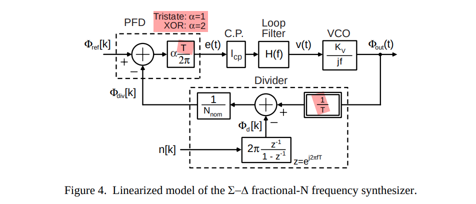
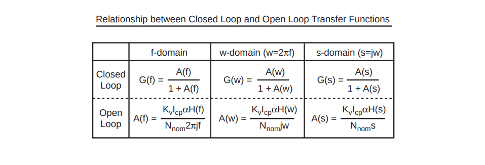
Michael H. Perrott, PLL Design Using the PLL Design Assistant Program. [https://designers-guide.org/forum/Attachments/pll_manual.pdf]
\(\frac{1}{T}\) & \(T\) come from CT-DT & DT-CT

H. Kang et al., "A 42.7Gb/s Optical Receiver With Digital Clock and Data Recovery in 28nm CMOS," in IEEE Access, vol. 12, pp. 109900-109911, 2024 [https://ieeexplore.ieee.org/stamp/stamp.jsp?tp=&arnumber=10630516]
Sonntag JSSC 2006
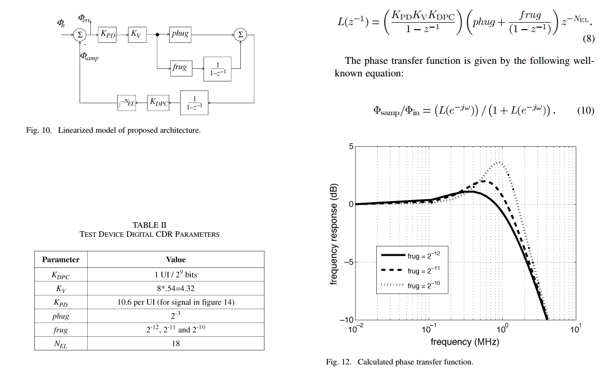
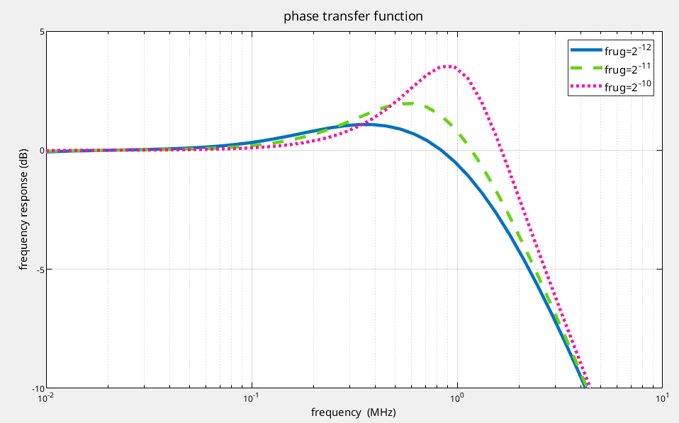
1 | clear; |
Full View
Kpd, Kb, Kv
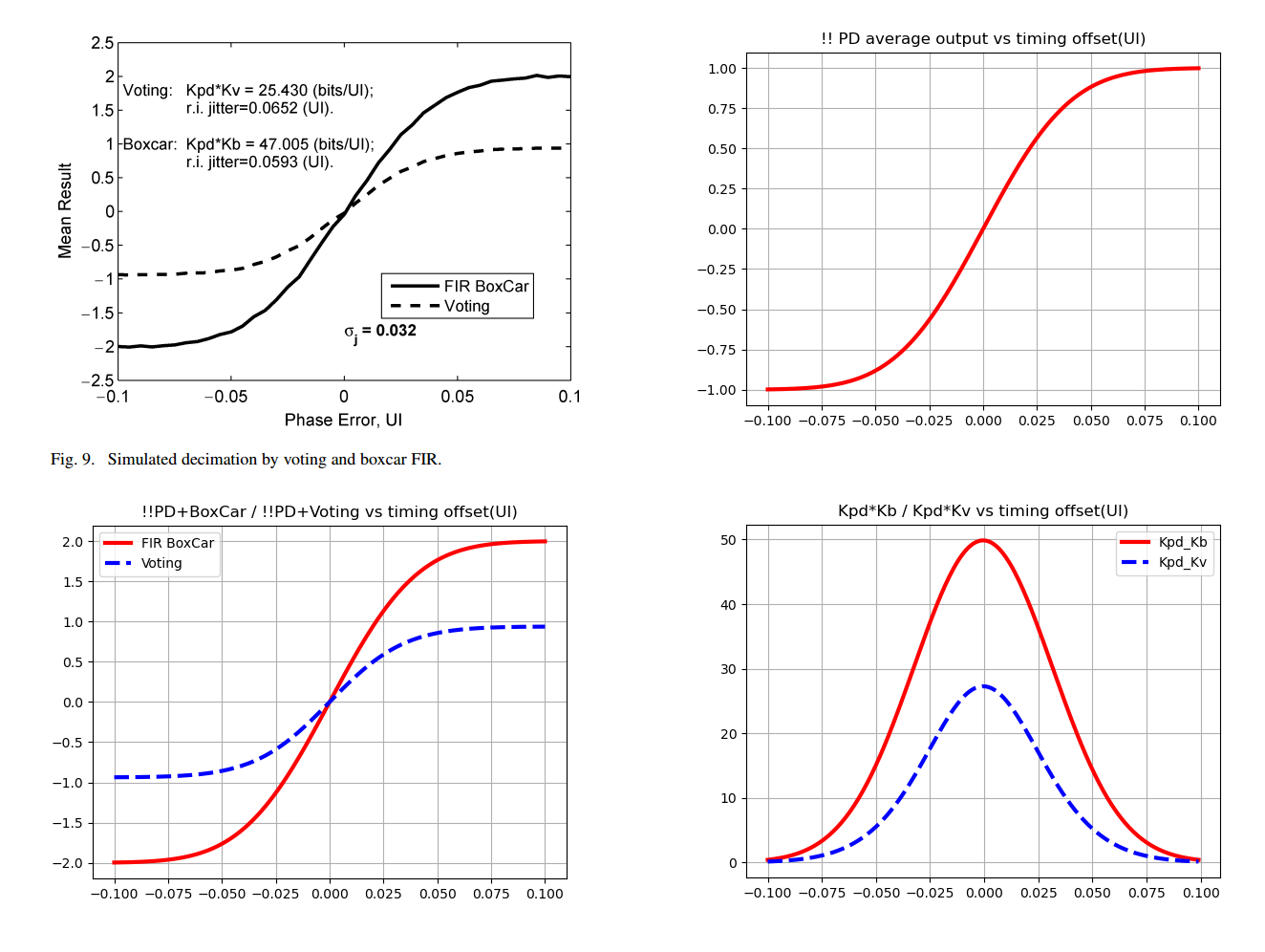
- Kpd formula: 12.467; Kpd_bb_0 12.465
- Kpd_Kb: 49.860; Kpd_Kv 27.265
- Kb: 4.00; Kv 2.19
That is
- gain of BoxCar is the decimation factor
- Voting across 4 inputs had a 54% reduced gain relative to boxcar filter
1 | import numpy as np |
with deci_factor = 8
1 | Kpd formula: 12.467; Kpd_bb_0 12.465 |
with deci_factor = 16
1 | Kpd formula: 12.467; Kpd_bb_0 12.465 |
reference
Alan V Oppenheim, Ronald W. Schafer. 2010. Discrete-Time Signal Processing, 3rd edition
R. E. Crochiere and L. R. Rabiner, "Multirate Digital Signal Processing", Prentice Hall, 1983.
John G. Proakis and Dimitris G. Manolakis, Digital Signal Processing: Principles, Algorithms, and Applications, 4th edition, 2007.
D. Sundararajan. 2024. Digital Signal Processing: An Introduction 2nd Edition
F. M. Gardner, "Phaselock Techniques", 3rd Edition, Wiley Interscience, Hoboken, NJ, 2005 [https://picture.iczhiku.com/resource/eetop/WyIgwGtkDSWGSxnm.pdf]
Rhee, W. (2020). Phase-locked frequency generation and clocking : architectures and circuits for modern wireless and wireline systems. The Institution of Engineering and Technology
Qasim Chaudhari. Sample Rate Conversion [https://wirelesspi.com/sample-rate-conversion/]
