Injection Locked Oscillators
Rotating Phasor
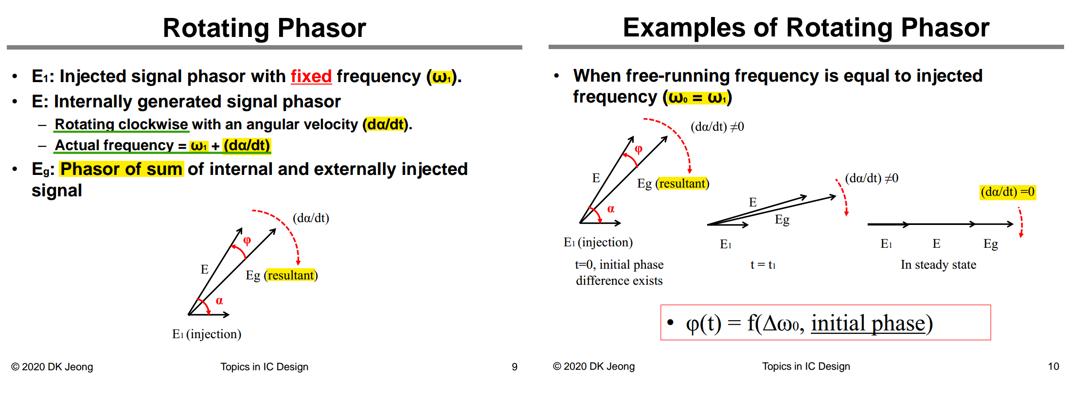
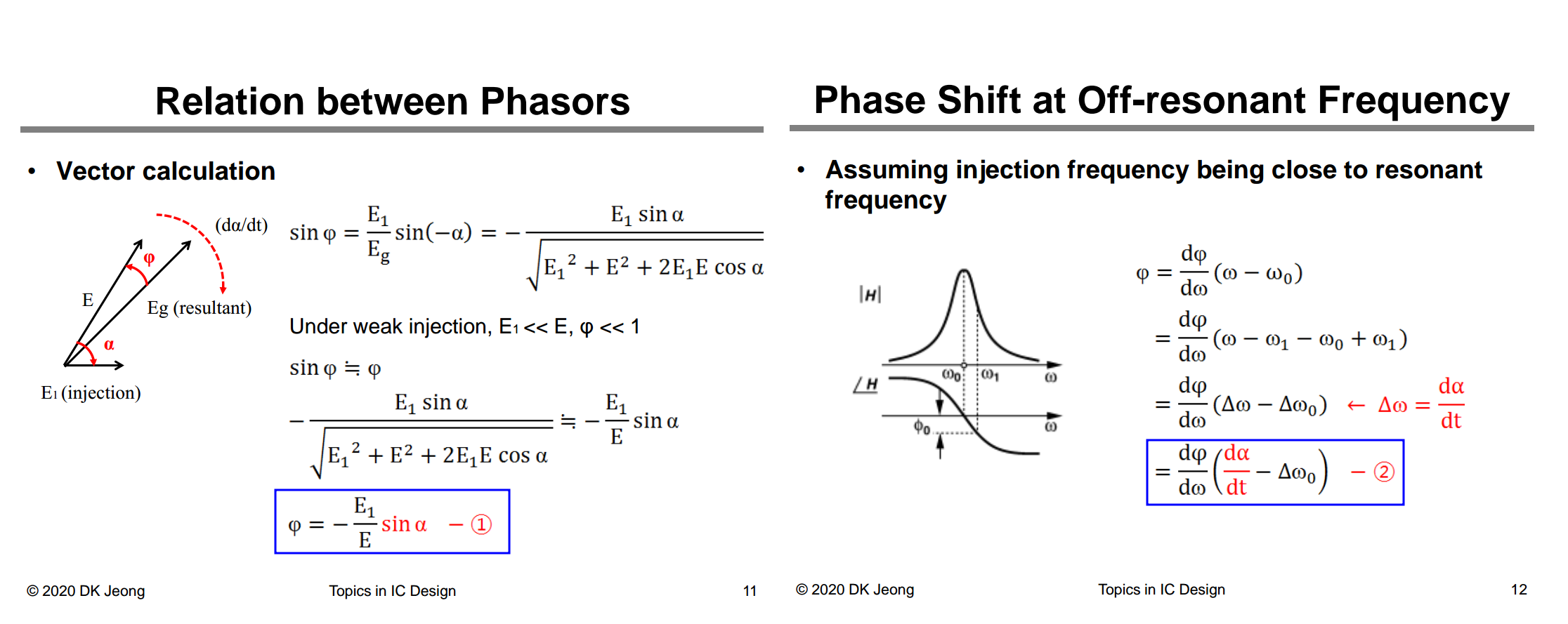
- \(E_1\): externally applied forcing signal.
- \(E\): oscillator-generated component after being influenced by \(E_1\).
- \(E_g\): total signal resulting from the oscillator-generated and injected contributions.
- \(\alpha(t)\) is the phase difference between the internal oscillator phasor \(E\), after being influenced by \(E_1\), and the injected phasor \(E_1\)
- \(\phi(t)\) is the angle between that internal oscillator phasor \(E\) and the resultant phasor \(E_g=E+E_1\)
Although \(E\) is called the "internally generated signal," it is not the free-running, unaffected signal. The coupling is implicit: \[ E_1 \rightarrow E_g=E+E_1 \rightarrow H(j\omega) \rightarrow E \] Therefore, \[ \boxed{E\text{ depends dynamically on }E_1.} \]
Adler's Equation
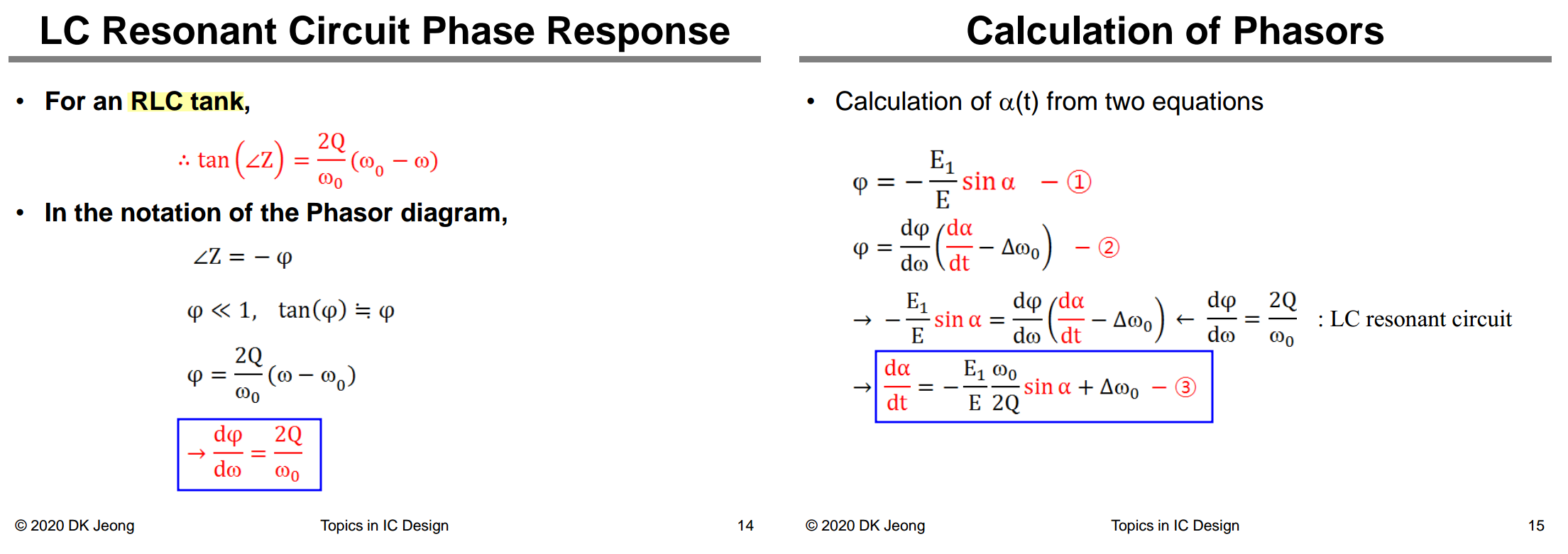
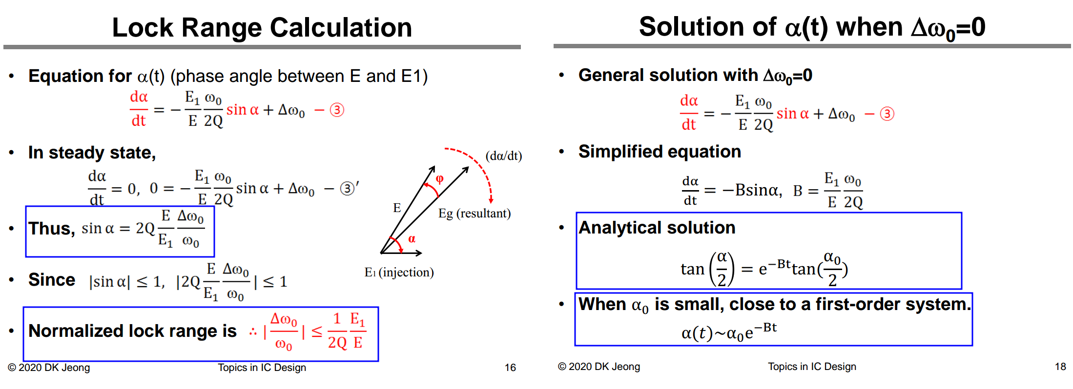
\[ \boxed{\frac{\mathrm{d}\alpha}{\mathrm{d}t} = \Delta\omega_0 - \frac{E_1}{E}\frac{\omega_0}{2Q}\sin\alpha} \] Define the injection-locking strength as \[ K = \frac{E_1}{E}\frac{\omega_0}{2Q}. \] Then Eq. (3) becomes the standard Adler form \[ \boxed{ \frac{\mathrm{d}\alpha}{\mathrm{d}t} = \Delta\omega_0-K\sin\alpha } \]
In steady state \[ \frac{\mathrm{d}\alpha}{\mathrm{d}t} = 0 \]
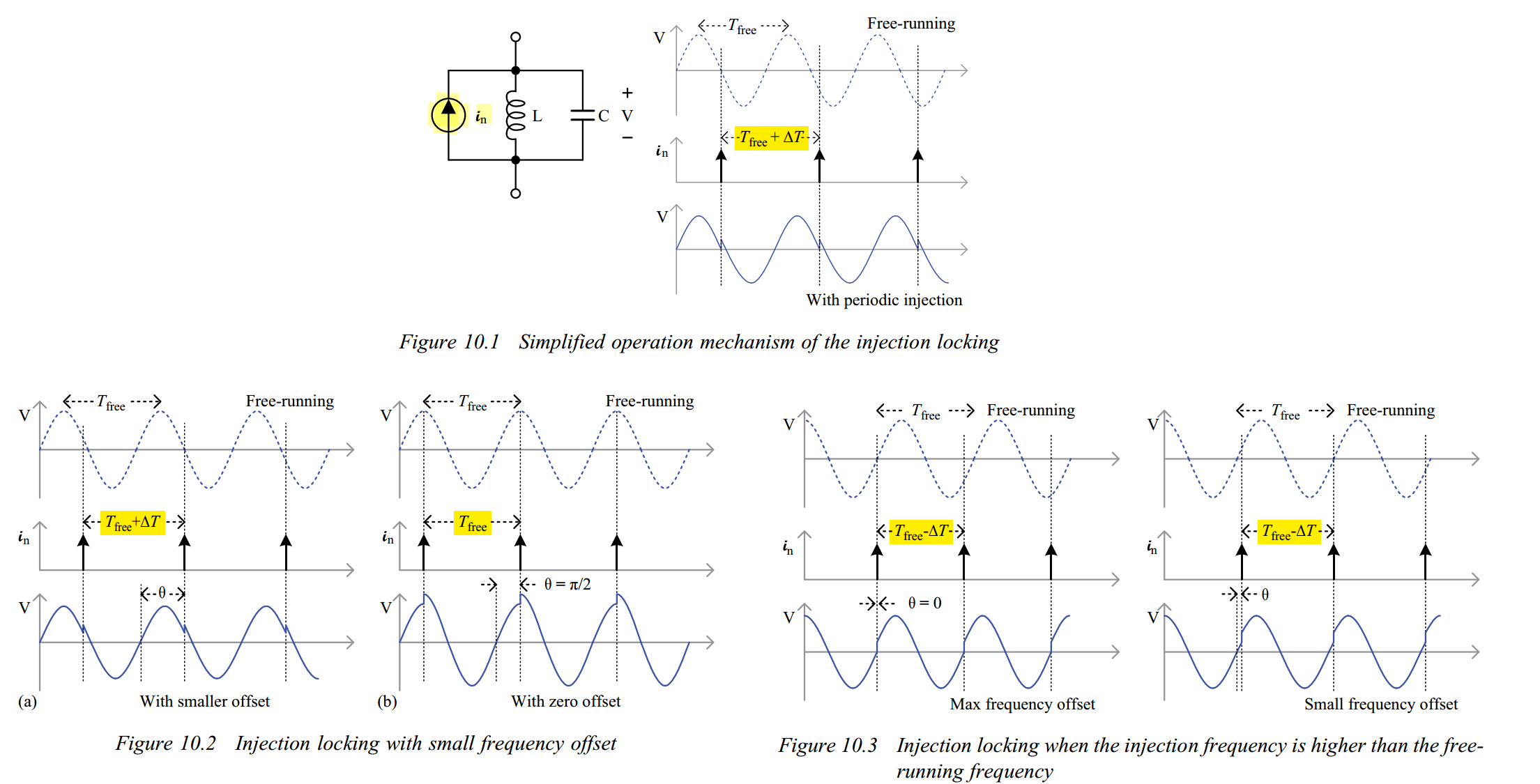
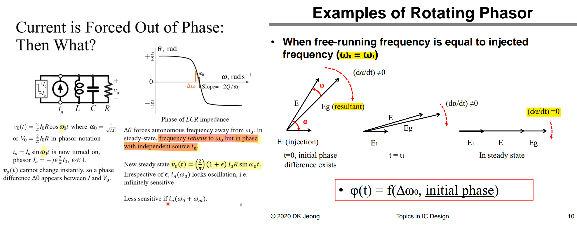
When free-running frequency is equal to injected frequency, in a steady state, the large oscillation aligns in phase with the small injected current
KCL plus the inductor law \[ C\dot v + \frac{v}{R} + i_L = \frac{\pi}{4}I_1\,\mathrm{sgn}(v) + \epsilon I_1\sin(\omega_{inj}t),\qquad L\,\dot i_L = v, \] with \(I_1\equiv\tfrac{2}{\pi}I_0\)
"inject at \(\omega_0\)" must mean the measured free-running frequency — we measure it from an \(\epsilon=0\) run first
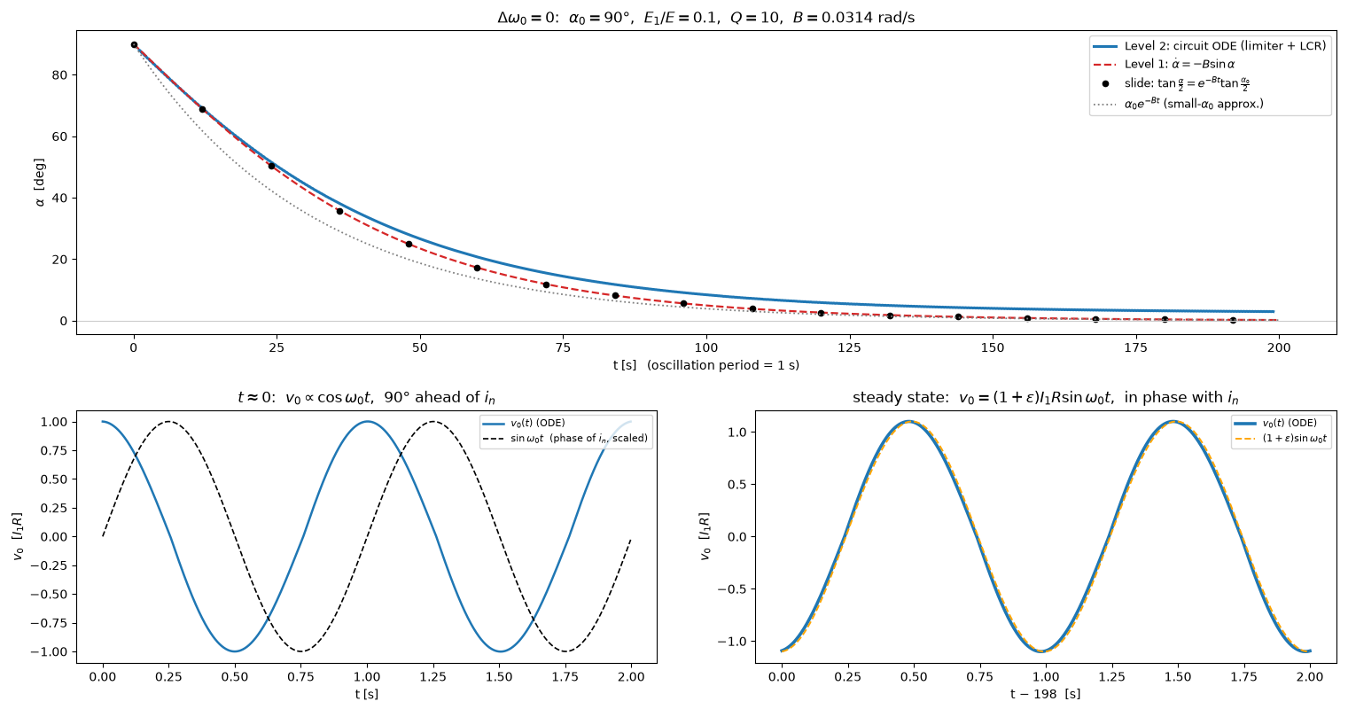
phase estimates the instantaneous phase of waveform
v relative to the reference \(\sin(\omega_{\rm ref}t)\)
It acts like a simple lock-in detector:
1 | N = int(round(2*np.pi / wref / dt)) |
Computes the number of samples in one reference period.
1 | Ic = moving_average(2*v*sin(wref*t)) |
The one-period moving average extracts the components of
v aligned with the reference sine and cosine while
suppressing harmonics.
For
\[ v(t)=A\sin(\omega_{\rm ref}t+\phi) \]
the averages are approximately
\[ I_c=A\cos\phi,\qquad Q_c=A\sin\phi \]
so:
1 | np.arctan2(Qc, Ic) |
returns \(\phi\), in radians between \(-\pi\) and \(\pi\)
1 | """ |
Fundamental ILO (1st harmonic)
TODO 📅
Subharmonic ILO
TODO 📅
Multiplying ILO (MILO)
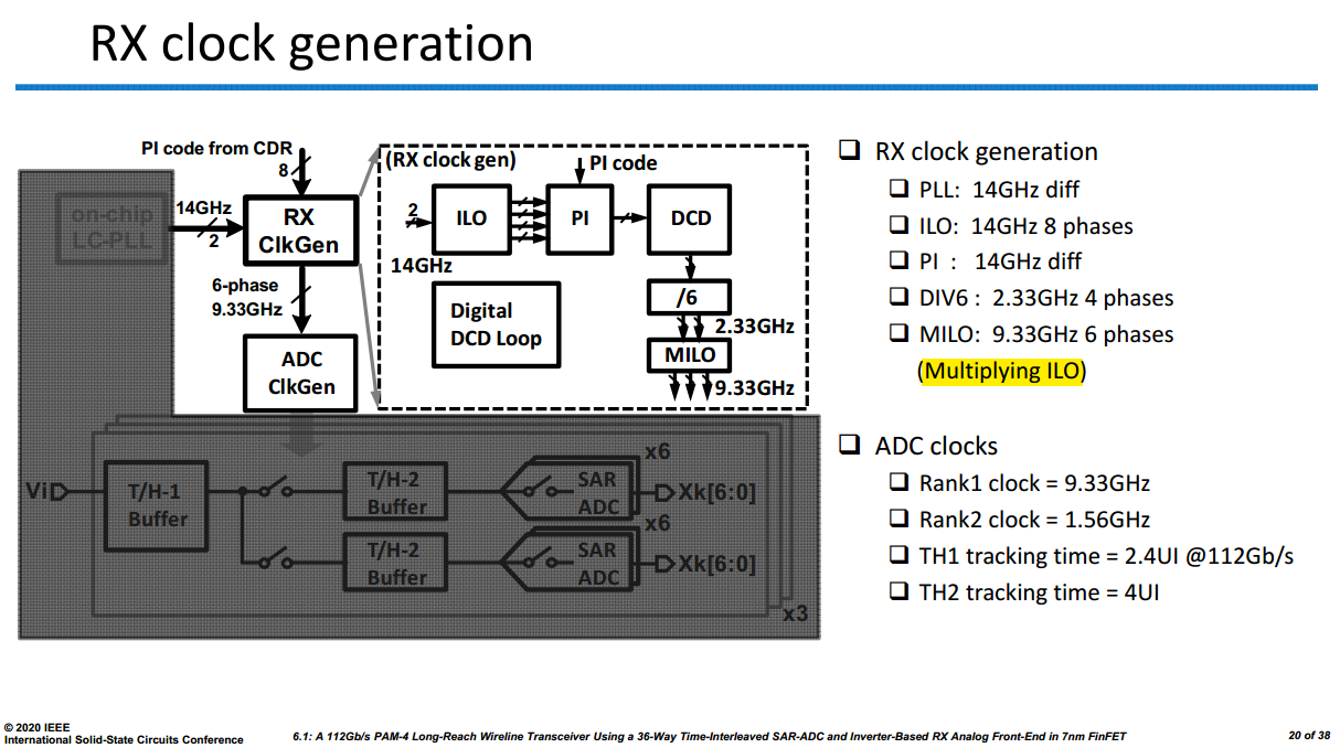
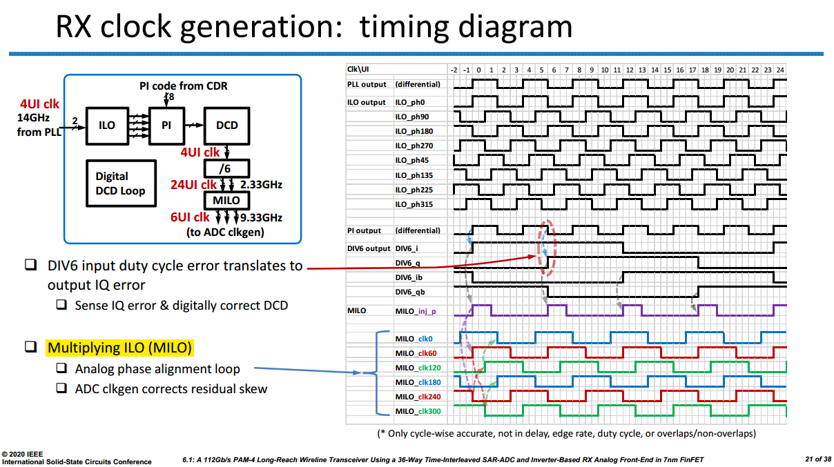
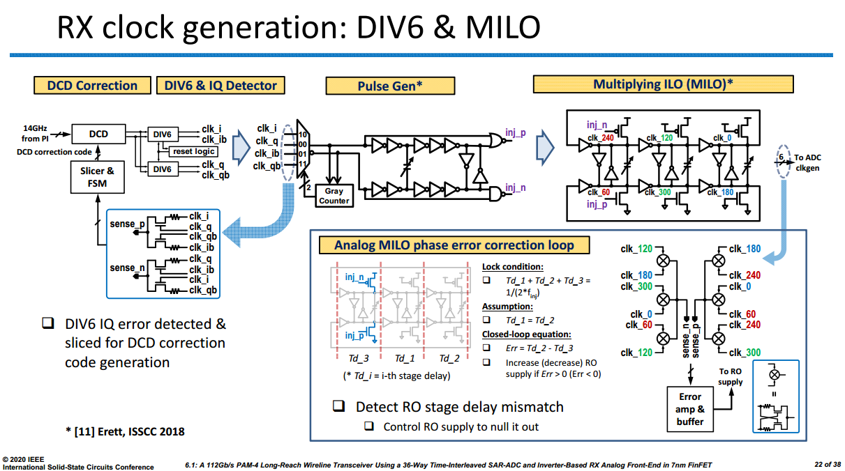
J. Im et al., "6.1 A 112Gb/s PAM-4 Long-Reach Wireline Transceiver Using a 36-Way Time-Interleaved SAR-ADC and Inverter-Based RX Analog Front-End in 7nm FinFET," 2020 IEEE International Solid-State Circuits Conference - (ISSCC), San Francisco, CA, USA, 2020, pp. 116-118 [https://sci-hub.ru/10.1109/ISSCC19947.2020.9063081]
M. Erett et al., "16.7 A 126mW 56Gb/s NRZ wireline transceiver for synchronous short-reach applications in 16nm FinFET," 2018 IEEE International Solid-State Circuits Conference - (ISSCC), San Francisco, CA, USA, 2018, pp. 274-276 [https://sci-hub.ru/10.1109/ISSCC.2018.8310290]
TODO 📅
reference
Bae, Woorham, and Deog-Kyoon Jeong. Analysis and Design of CMOS Clocking Circuits for Low Phase Noise. Institution of Engineering and Technology, 2020
Cowan, Glenn. (2024). Mixed-Signal CMOS for Wireline Communication: Transistor-Level and System-Level Design Considerations
R. Adler, "A Study of Locking Phenomena in Oscillators," in Proceedings of the IRE, vol. 34, no. 6, pp. 351-357, June 1946 [https://sci-hub.jp/10.1109/JRPROC.1946.229930]
—, "A study of locking phenomena in oscillators," in Proceedings of the IEEE, vol. 61, no. 10, pp. 1380-1385, Oct. 1973 [https://sci-hub.jp/10.1109/PROC.1973.9292]
B. Razavi, "A study of injection locking and pulling in oscillators," in IEEE Journal of Solid-State Circuits, vol. 39, no. 9, pp. 1415-1424, Sept. 2004 [https://www.seas.ucla.edu/brweb/papers/Journals/RSep04.pdf]
A. A. Hafez and C. -K. K. Yang, "Analysis and Design of Superharmonic Injection-Locked Multipath Ring Oscillators," in IEEE Transactions on Circuits and Systems I: Regular Papers, vol. 60, no. 7, pp. 1712-1725, July 2013 [https://sci-hub.ru/10.1109/TCSI.2012.2230591]
Deog-Kyoon Jeong. "Topics in IC (Wireline Transceiver Design): Lec 4 - Injection Locked Oscillators" [https://ocw.snu.ac.kr/sites/default/files/NOTE/Lec%204%20-%20Injection%20Locked%20Oscillators.pdf]
Min-Seong Choo. Review of Injection-Locked Oscillators [https://journal.theise.org/jse/wp-content/uploads/sites/2/2020/09/JSE-2020-0001.pdf]
Mozhgan Mansuri. ISSCC2021 SC3: Clocking, Clock Distribution, and Clock Management in Wireline/Wireless Subsystems
Aditya Varma Muppala. Oscillator Theory - Injection Locking [note, video1, video2]
Ali M. Niknejad. EECS 242 Lecture 26 Injection Locking [https://rfic.eecs.berkeley.edu/courses/ee242/pdf/eecs242_lect26_injectionlocking.pdf]
Tony Chan Carusone, 35 Injection Locked Oscillators [https://youtu.be/IgB2NRdUMVo]