Crosstalk in Transmission Lines
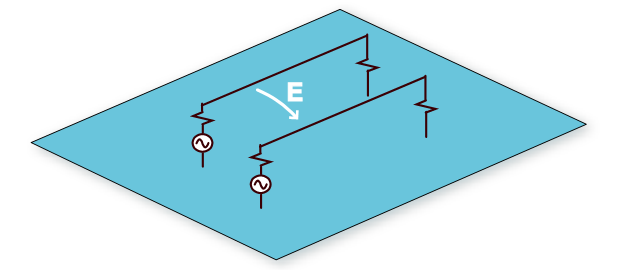
Electric field coupling (also called capacitive coupling) occurs when energy is coupled from one circuit to another through an electric field
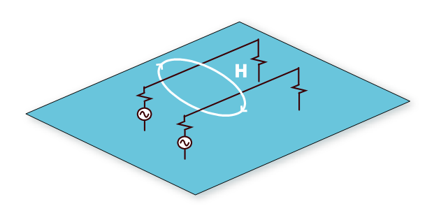
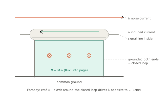
Magnetic field coupling (also called inductive coupling) occurs when energy is coupled from one circuit to another through a magnetic field
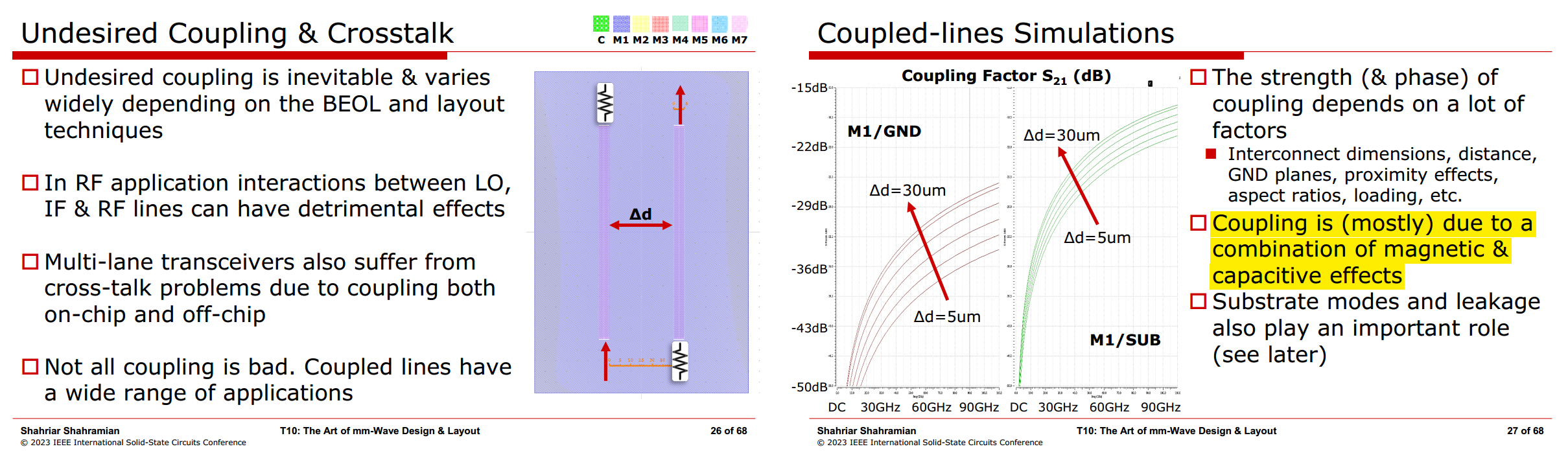
For instance
- magnetic coupling between multiple inductors
- capacitive coupling between multiple transmission lines
Transmission Line
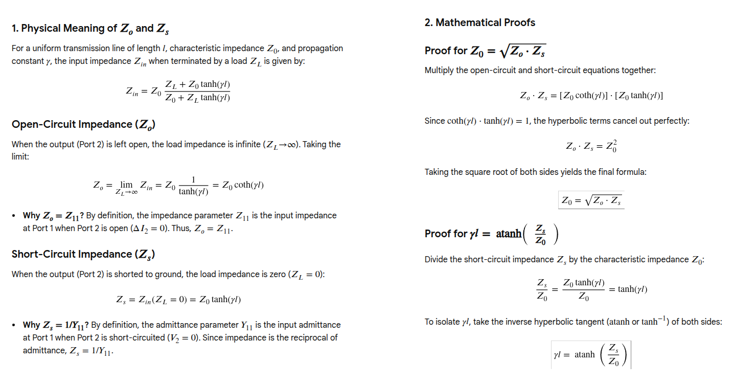
param. extraction from ABCD matrix
Chapter 4.5. High Frequency Passive Devices [https://www.cambridge.org/il/files/7713/6698/2369/HFIC_chapter_4_passives.pdf]
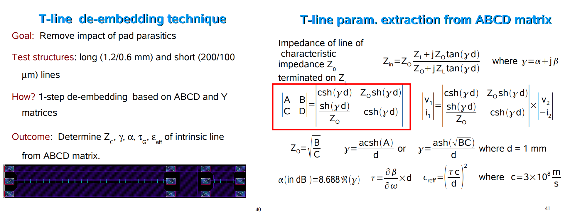
for lossless T-line, \(\gamma = j\beta\)

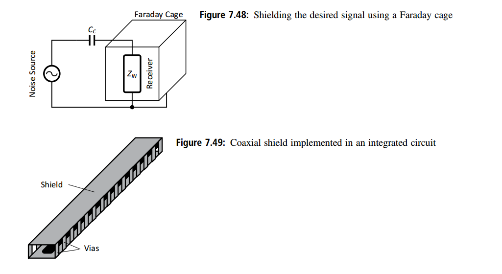
Capacitive Coupling
Faraday cage
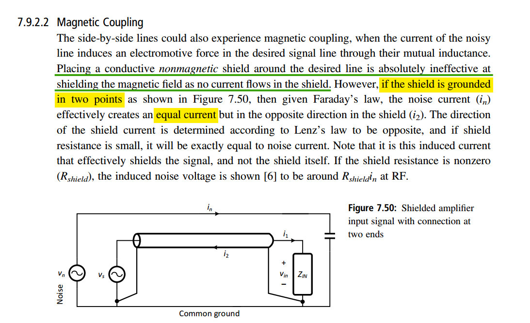
Magnetic Coupling
Darabi H. Radio Frequency Integrated Circuits and Systems. 2nd ed. Cambridge University Press; 2020.
NEXT & FEXT
Backward (near-end) crosstalk & Forward (far-end) crosstalk
Mohammad Abu Khater, ISCAS2019 tutorial: High-Performance Printed Circuit Boards (PCBs)
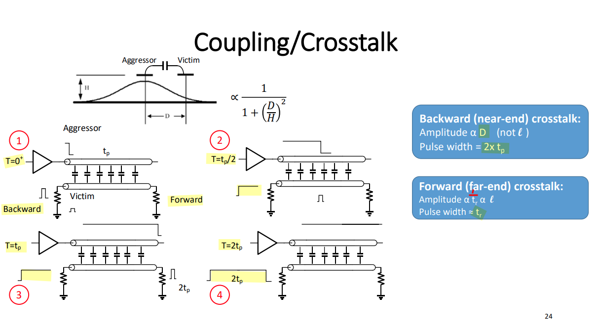
Consider a small section at distance (x) from the input:
- The aggressor’s edge reaches it at time \(x/v\), generating a small noise pulse.
- That pulse travels forward on the victim through the remaining distance \(\ell-x\)
Its arrival time at the far end is therefore
\[ t_{\text{arrival}} =\underbrace{\frac{x}{v}}_{\text{aggressor reaches section}} +\underbrace{\frac{\ell-x}{v}}_{\text{noise reaches far end}} =\frac{\ell}{v} \]
Noise generated earlier travels farther; noise generated later travels less. The pulses overlap, so adding more coupled sections increases their summed amplitude
Each short section contributes in proportion to its length and the edge slope: \[ dV_F\propto dx\,\frac{\Delta V}{t_r} \quad\Longrightarrow\quad \boxed{V_{F,\text{peak}}\propto \ell\,\frac{\Delta V}{t_r}} \]
Here, \(\ell\) means the length over which the traces run alongside each other.
For comparison, backward noise arrives at \(x/v+x/v=2x/v\), so contributions from different locations spread out in time. That explains why extending a sufficiently long coupled line mainly increases the backward pulse’s duration
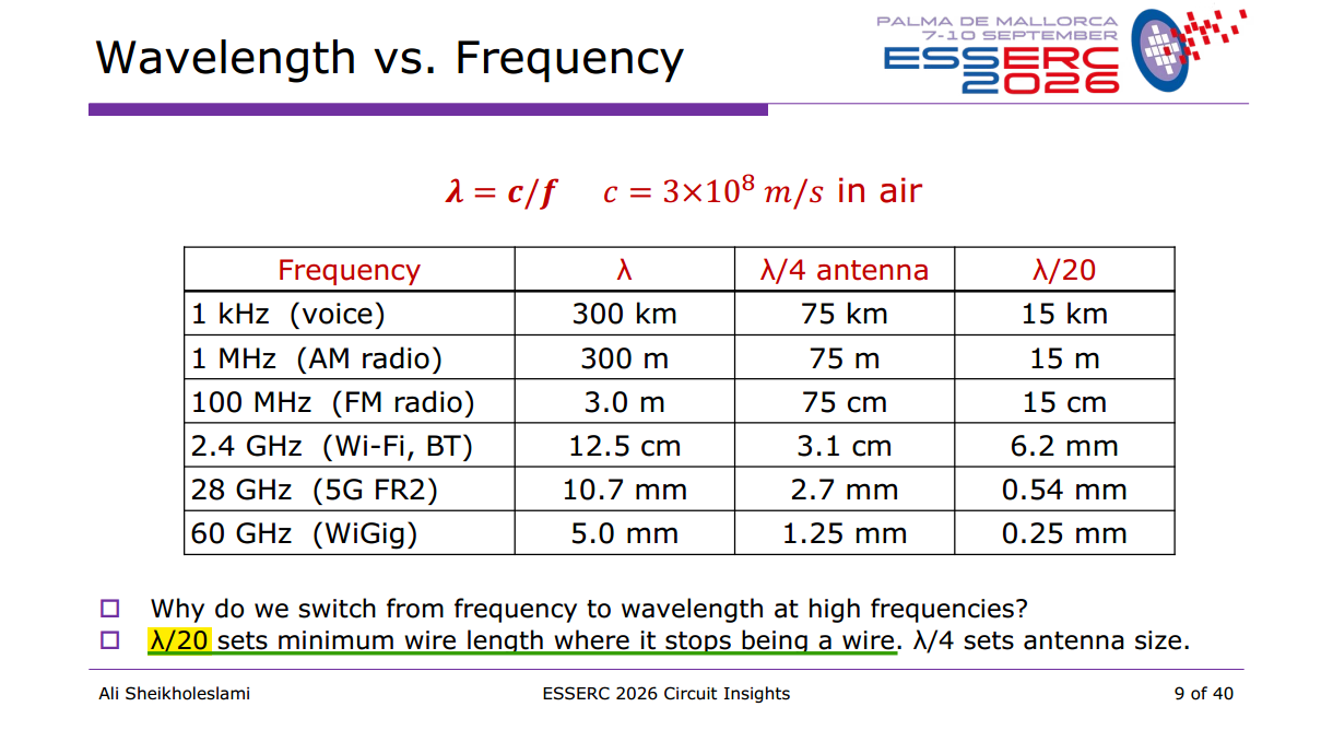
Wavelength vs. Frequency
Ali Sheikholeslami, ESSERC 2026 Circuit Insights: Fundamentals of Circuit Design at High Frequencies
relative dielectric constant vs permittivity
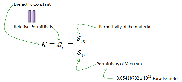
The relative dielectric constant characterizes some of the electrical properties of an insulator
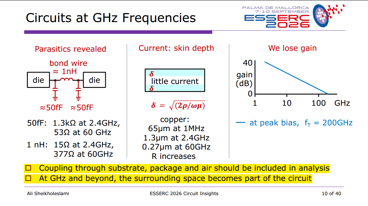
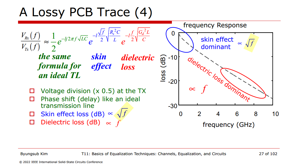
skin effect & Dielectric loss
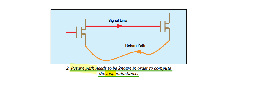
Return Path
ISSCC2002. Special Topic Evening Discussion Sessions SE1: Inductance: Implications and Solutions for High-Speed Digital Circuits [vSE1_Blaauw], [vSE1_Gauthier], [vSE1_Morton, [vSE1_Restle]]
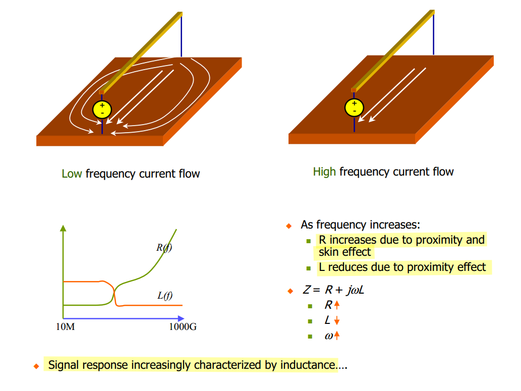
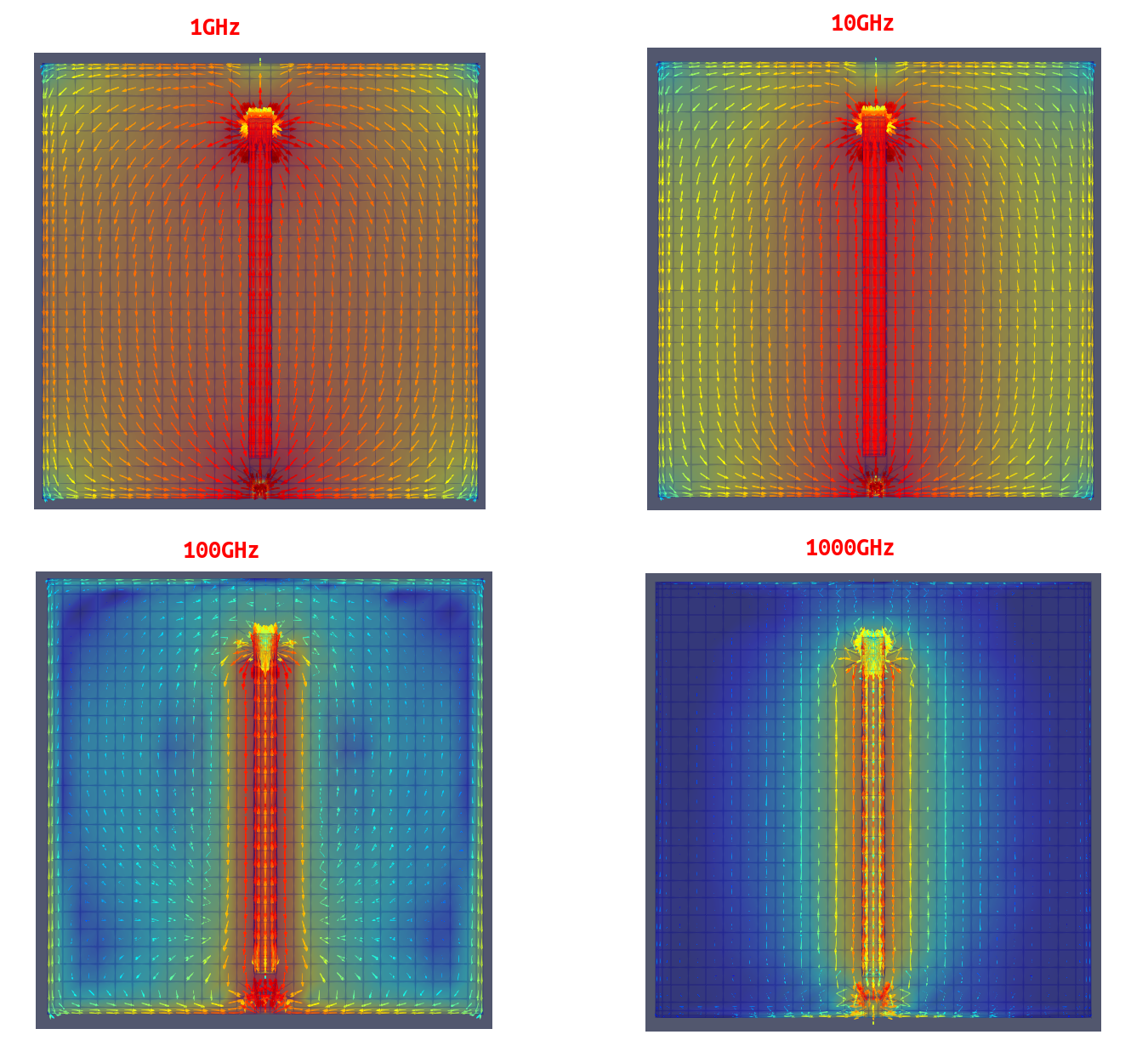
Current return paths are frequency dependent \(Z = R +j\omega L\)
- Low frequency
- \(R\) dominates - current use as many returns as possible to have parallel resistances
- High frequency
- \(j\omega L\) dominates - current use the closest possible return path to form the smallest possible loop inductance
- Very high frequency
- The current would be confined to the nearest possible return only at ultra-high frequencies (skin effect)
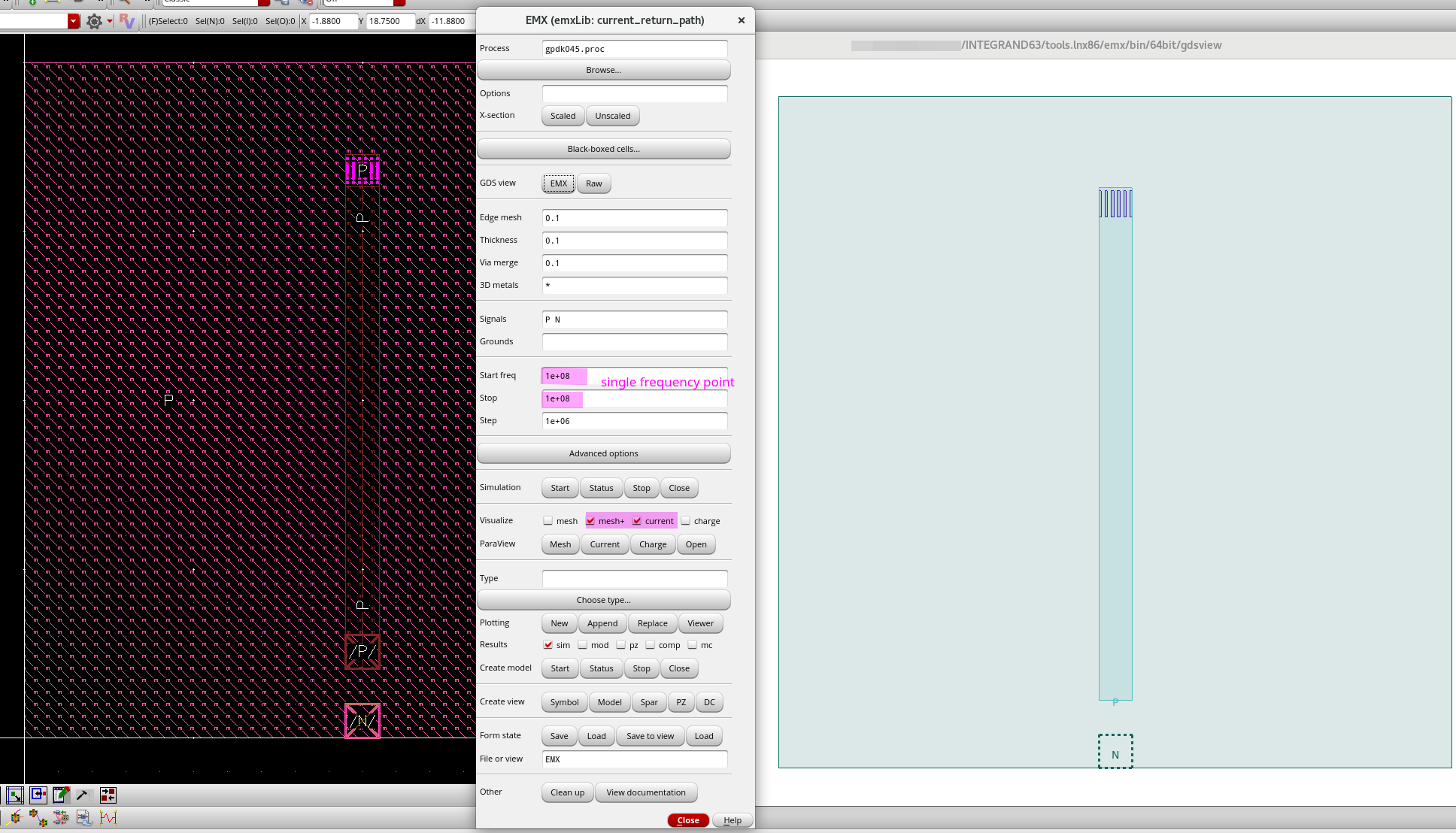
EMX simulation
setup:
frequency sweep:
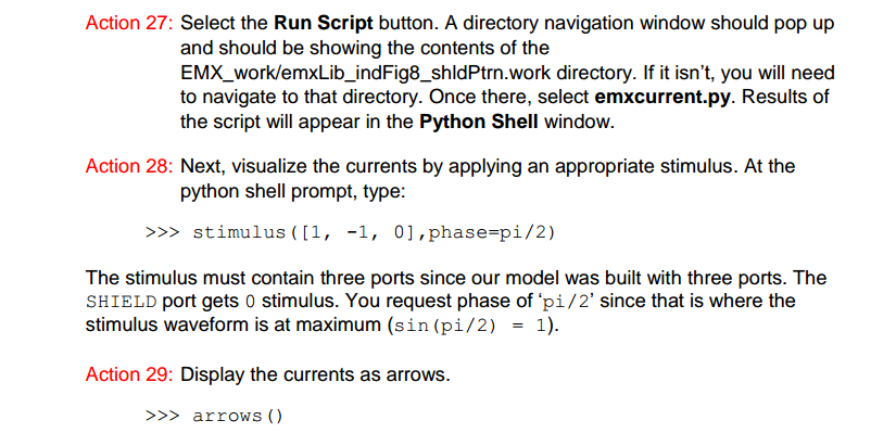
Cadence October 2020, Analysis of a Figure-Eight Inductor with EMX RAK
Tline Approximation
[https://web.stanford.edu/class/archive/ee/ee371/ee371.1066/handouts/markChapt.pdf]
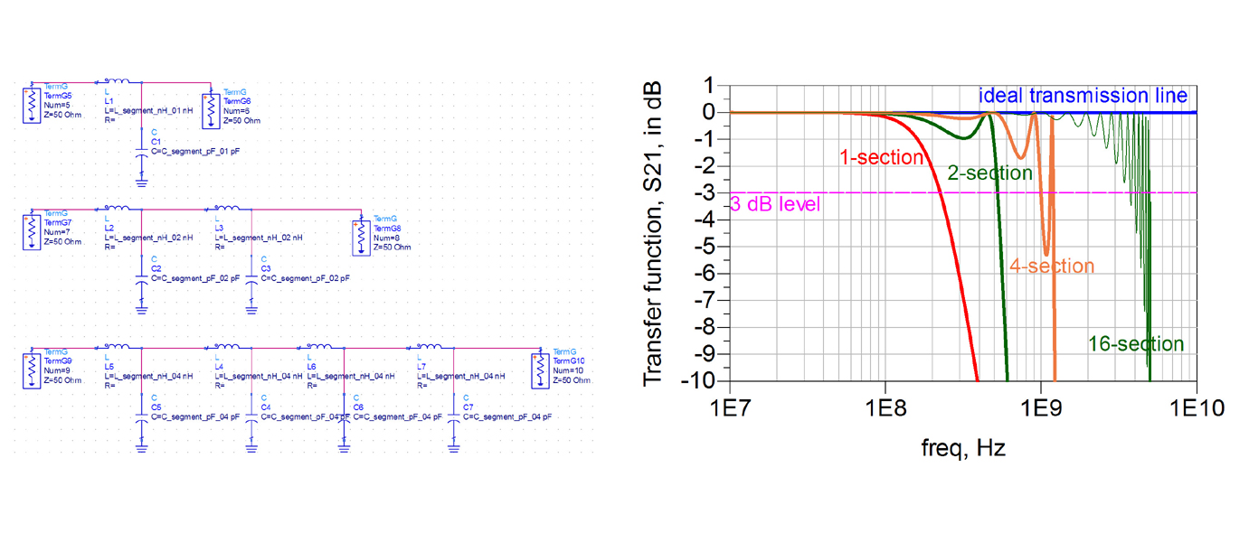
N-section LC Model
Eric Bogatin. Pop Quiz: When is an Interconnect Not a Transmission Line? [https://www.signalintegrityjournal.com/blogs/4-eric-bogatin-signal-integrity-journal-technical-editor/post/265-pop-quiz-when-is-an-interconnect-not-a-transmission-line]

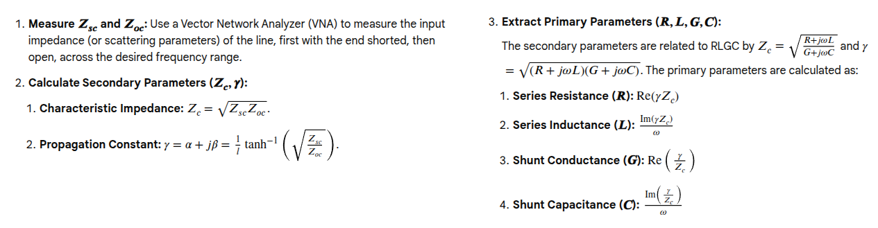
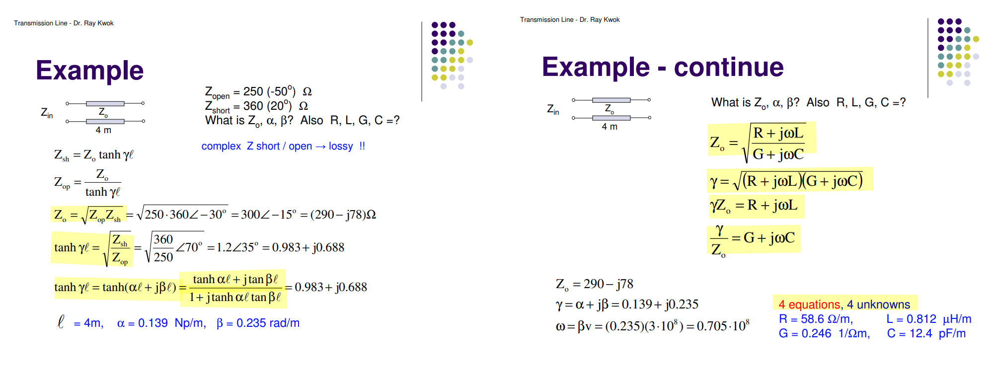
RLGC by Open/Short Circuit
RLGC can be extracted from measurements of a transmission line's input impedance under open-circuit and short-circuit terminations at a specific frequency
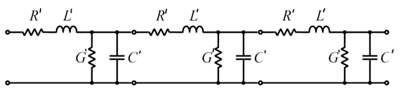
Dr. Muehlhaus Consulting & Software GmbH, lumpedmodel [https://github.com/VolkerMuehlhaus/lumpedmodel]
Transmission line from S2P data into RLGC lumped model
 \[
\boxed{R= \text{Re}(\gamma Z_c)} \qquad
\boxed{L= \frac{\text{Im}(\gamma Z_c)}{\omega}} \qquad
\boxed{G= \text{Re}\left(\frac{\gamma}{Z_c}\right)} \qquad
\boxed{C= \frac{\text{Im}\left(\frac{\gamma}{Z_c}\right)}{\omega}}
\]
\[
\boxed{R= \text{Re}(\gamma Z_c)} \qquad
\boxed{L= \frac{\text{Im}(\gamma Z_c)}{\omega}} \qquad
\boxed{G= \text{Re}\left(\frac{\gamma}{Z_c}\right)} \qquad
\boxed{C= \frac{\text{Im}\left(\frac{\gamma}{Z_c}\right)}{\omega}}
\]
1 | # https://github.com/VolkerMuehlhaus/lumpedmodel/blob/main/rlgc_from_s2p/rlgc_from_s2p.py |
Transmission Line [pdf]
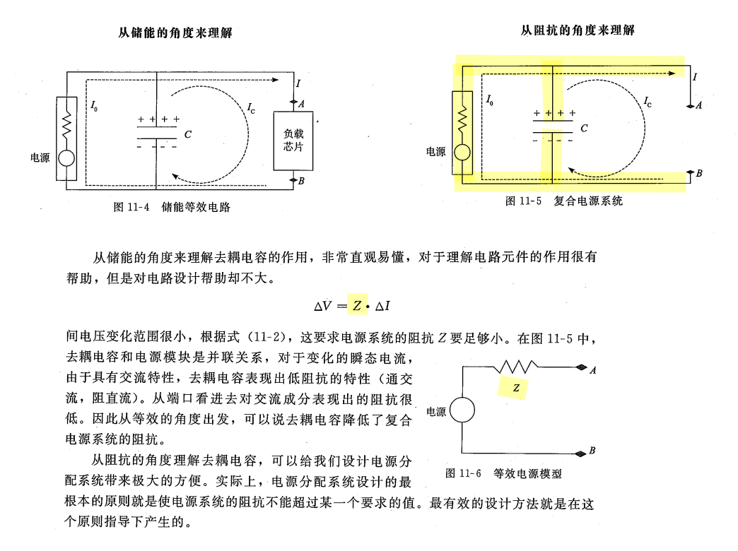
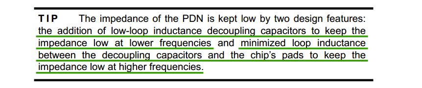
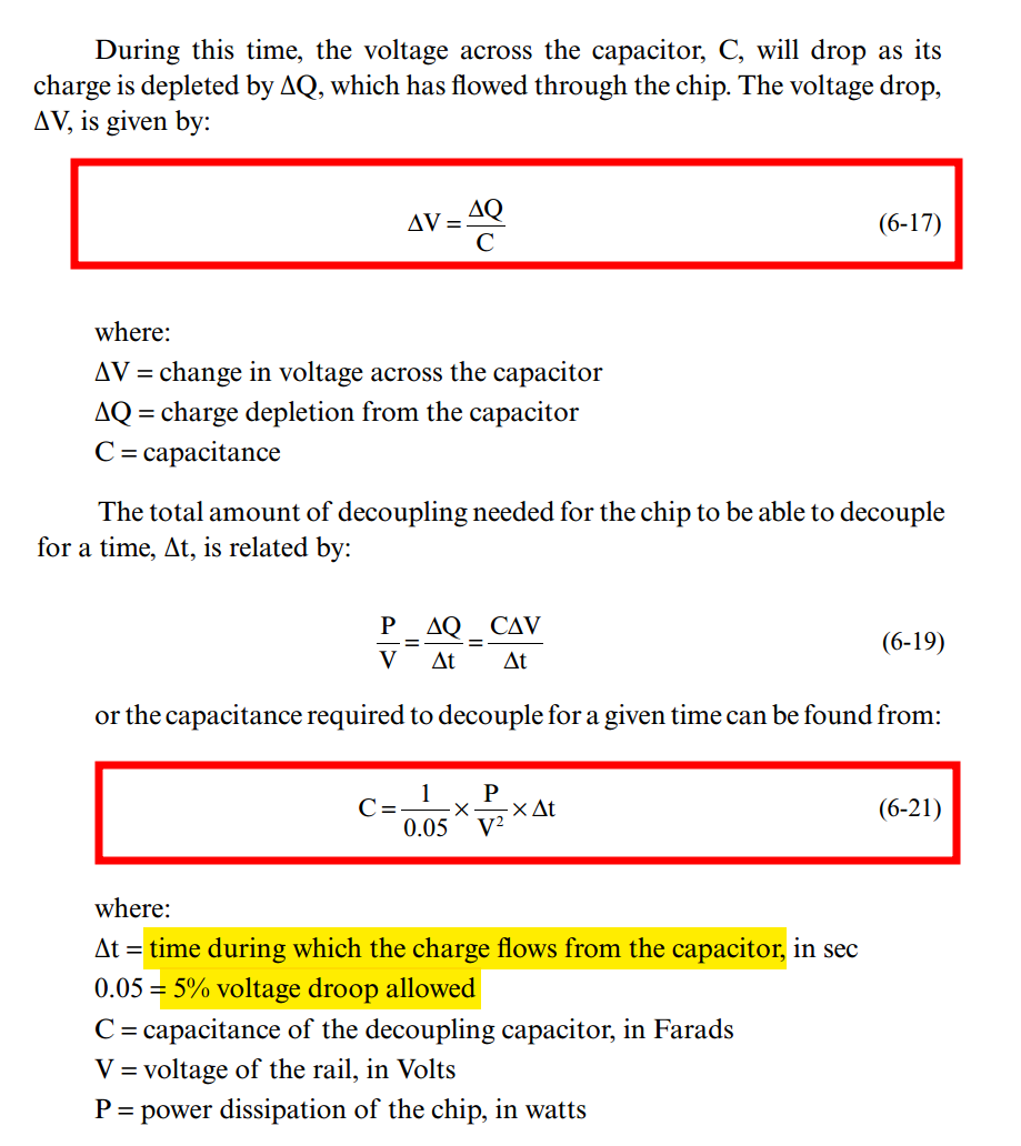
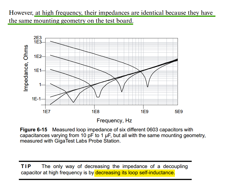
Decoupling Capacitor
Grounding
Chapter 11 Layout and grounding [http://ieb-srv1.upc.es/gieb/tecniques/doc/EMC/pdfs/ScienceDirect_articles_27Jul2018_12-16-10.699/Chapter-11---Layout-and-grounding_2007_EMC-for-Product-Designers.pdf]
TODO
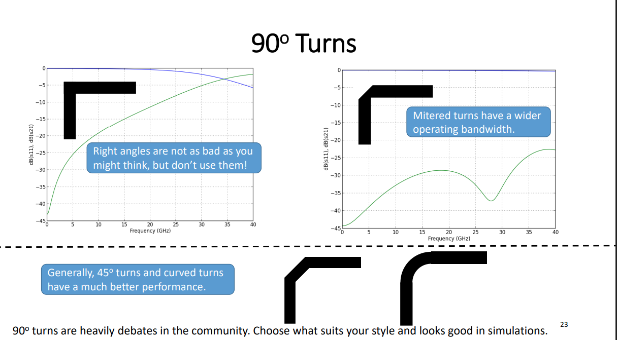
90o Turns
Mohammad Abu Khater, ISCAS2019 tutorial: High-Performance Printed Circuit Boards (PCBs)
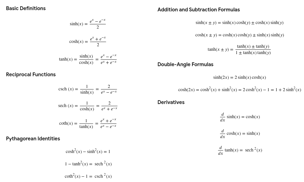
Hyperbolic Functions
reference
信号完整性揭秘:于博士SI设计手记
Bogatin, E. (2018). Signal and power integrity, simplified. Prentice Hall. [pdf]
High-speed Serial Interface Lect. 9 – Noise [http://tera.yonsei.ac.kr/class/2017_2_2/lecture/Lect%209%20Noise.pdf]
Yuriy Shlepnev. How Interconnects Work: Characteristic Impedance and Reflections [https://www.linkedin.com/pulse/how-interconnects-work-characteristic-impedance-yuriy-shlepnev/]
—. How Interconnects Work: Bandwidth for Modeling and Measurements [https://www.linkedin.com/pulse/how-interconnects-work-bandwidth-modeling-yuriy-shlepnev/?trackingId=874kpm3XuNyV9D0eP6IioA%3D%3D]
Eric Bogatin. Pop Quiz: When is an Interconnect Not a Transmission Line? [https://www.signalintegrityjournal.com/blogs/4-eric-bogatin-signal-integrity-journal-technical-editor/post/265-pop-quiz-when-is-an-interconnect-not-a-transmission-line]
TeledyneLeCroy/SignalIntegrity Python tools for signal integrity applications [SignalIntegrityApp]
A Look at Transmission-Line Losses [http://blog.teledynelecroy.com/2018/06/a-look-at-transmission-line-losses.html]
How Much Transmission-Line Loss is Too Much? [http://blog.teledynelecroy.com/2018/06/how-much-transmission-line-loss-is-too.html]
Raymond Y. Chen, Raymond Y. Chen. Fundamentals of S Fundamentals of S-Parameter Parameter Modeling for Power Distribution Modeling for Power Distribution System (PDS) and SSO Analysis System (PDS) and SSO Analysis [https://ibis.org/summits/jun05/chen.pdf]
Sam Palermo, ECEN720: High-Speed Links Circuits and Systems Spring 2025 Lecture 9: Noise Sources [https://people.engr.tamu.edu/spalermo/ecen689/lecture9_ee720_noise_sources.pdf]