Decimation and Interpolation Filters
Decimation Filter
[https://web.engr.oregonstate.edu/~temes/ece627/Lecture_Notes/First_Order_DS_ADC_scan1.pdf]
[https://web.engr.oregonstate.edu/~temes/ece627/Lecture_Notes/First_Order_DS_ADC_scan2.pdf]
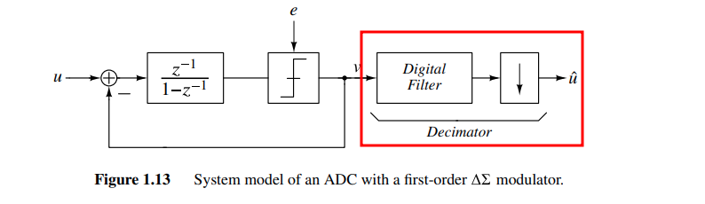
The combination of the the digital post-filter and downsampler is called the decimation filter or decimator
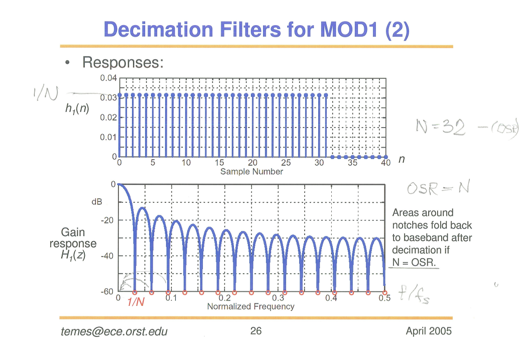
\(\text{sinc}\) filter
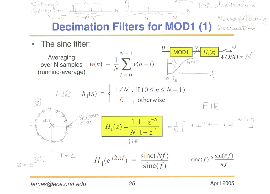
Suppose \(T=1\) \[ H_1(e^{j2\pi f}) = \frac{\text{sinc}(Nf)}{\text{sinc}(f)} = \frac{1}{N}\frac{\sin(\pi Nf)}{\sin(\pi f)} \] that is \(\lim_{f\to 0^+}H_1(e^{j2\pi f}) = 1\) and \(H_1 = 0\) when \(f=\frac{n}{N}, n\in \mathbb{Z}\)
A Beginner's Guide To Cascaded Integrator-Comb (CIC) Filters [https://www.dsprelated.com/showarticle/1337.php]
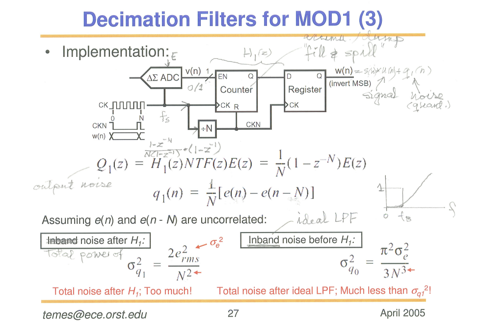
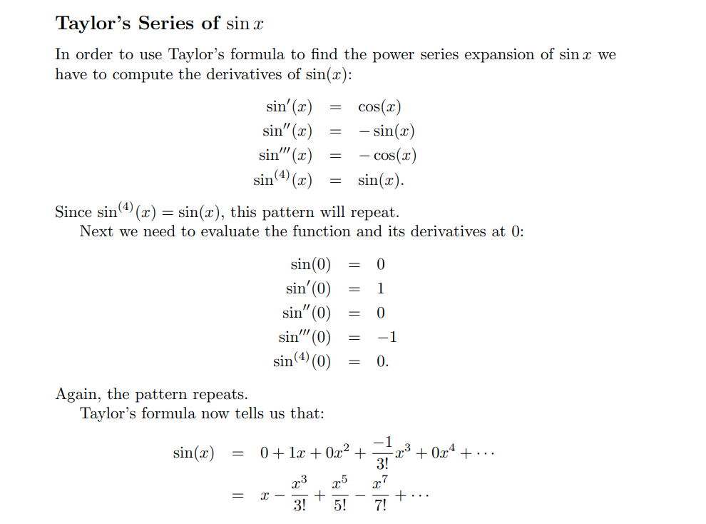
\[ |H_1(\omega)|^2 = \left|\frac{1}{N}(1-e^{-j\omega N}) \right| = \frac{2}{N^2}(1-\cos (\omega N)) \] Total noise after \(H_1\) \[ \sigma_{q_1}^2 = 2\int_0^\pi \frac{e^2_{rms}}{2\pi}\cdot |H_1(\omega)|^2d\omega = \frac{2e^2_{rms}}{N^2} \] inband noise before \(H_1\), i.e. ideal LPF with cutoff frequency \(\frac{\pi}{N}\) \[ \sigma_{q_0}^2 = 2\int_0^{\pi/N}\frac{e_{rms}^2}{2\pi}|1-e^{-j\omega}|^2d\omega = \frac{2e_{rms}^2}{\pi}\left(\frac{\pi}{N}-\sin\frac{\pi}{N}\right) \] with Taylor series \(\sin\frac{\pi}{N}\approx \frac{\pi}{N}-\frac{1}{6}\frac{\pi^3}{N^3}\) \[ \sigma_{q_0}^2 \approx \frac{\pi^2}{3N^3}e_{rms}^2 \]
Taylor’s Series of \(\sin x\) [pdf]
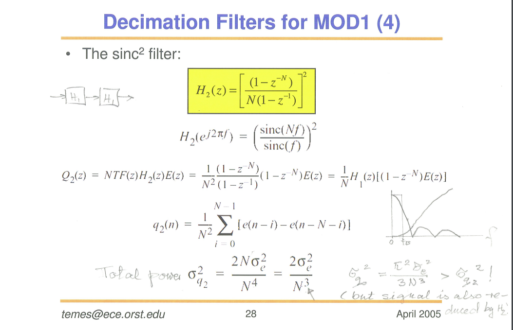
\(\text{sinc}^2\) filter
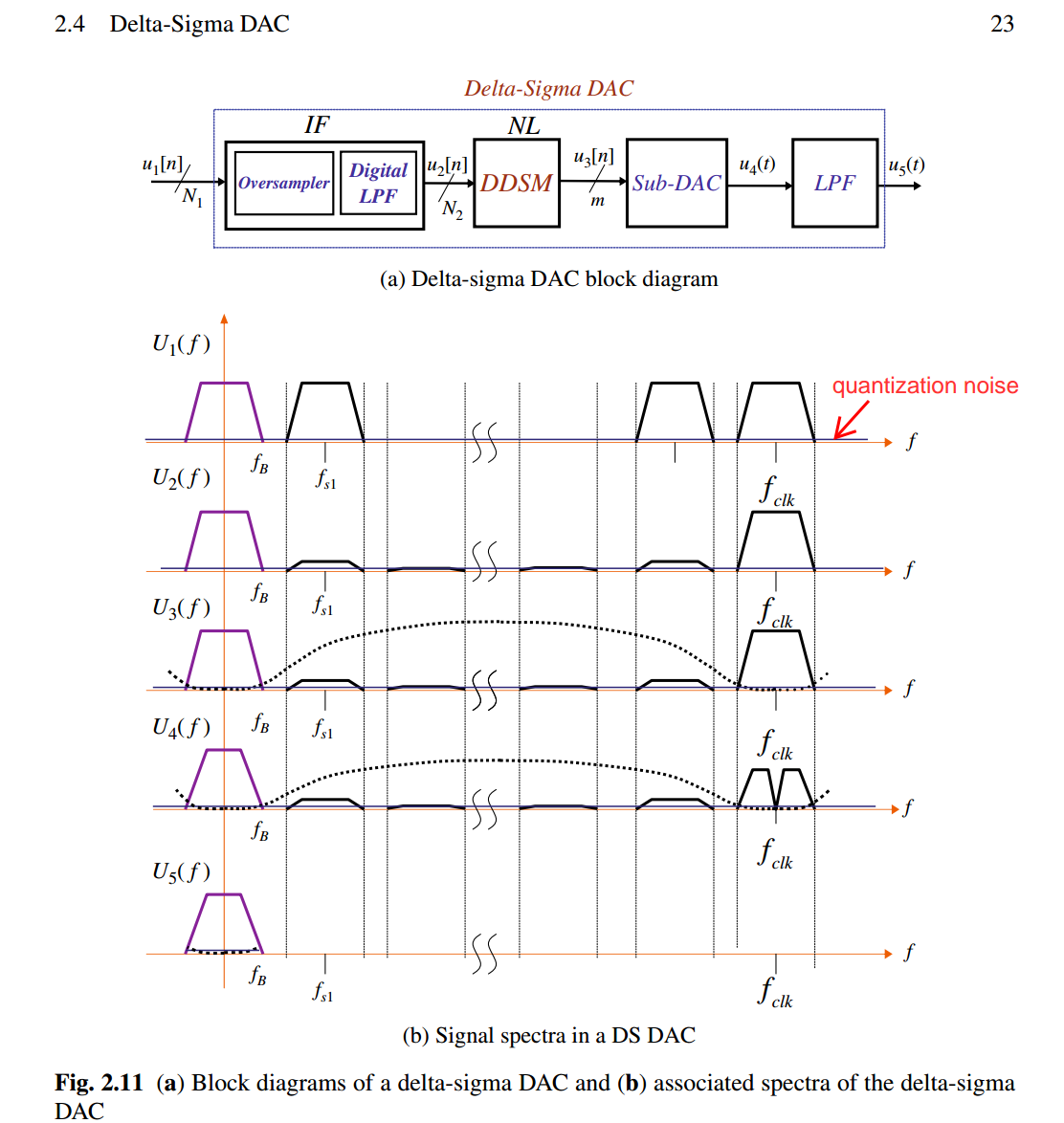
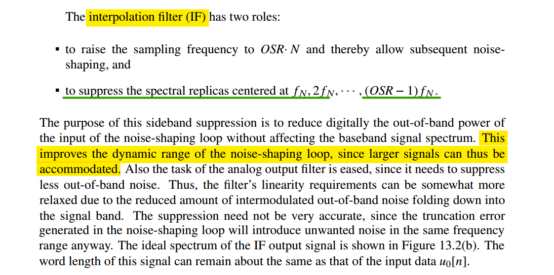
Interpolation Filter
Notice that the requirements of the first stage are very demanding
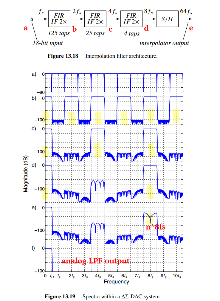
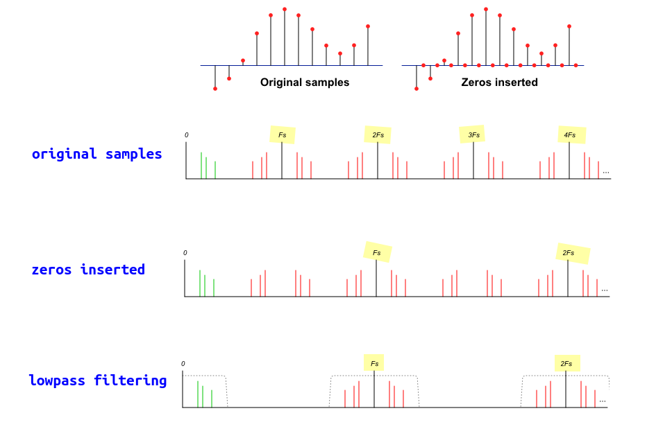
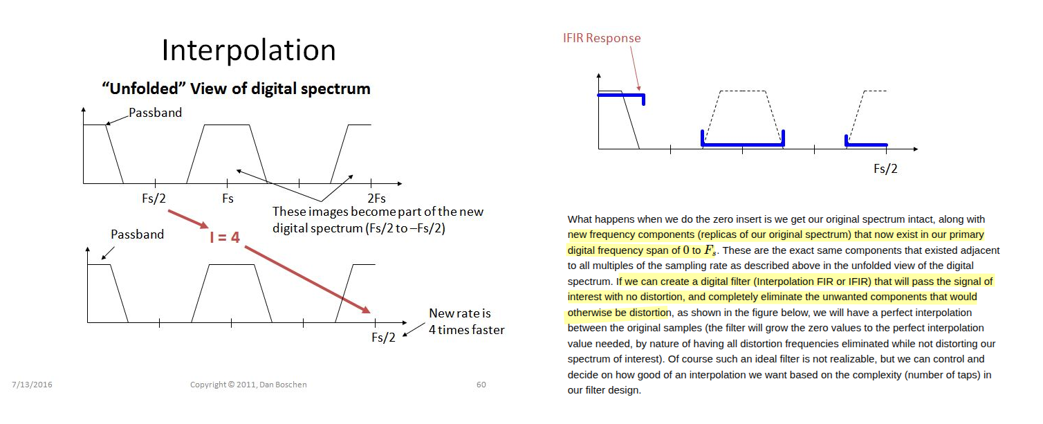
replicas suppression
The spectrum of the high resolution digital signal \(u_1\) contains the original baseband portion and its replicas located at integer multiples of \(f_{s1}\), plus a small amount of quantization noise shown as a solid line
Nigel Redmon [https://dsp.stackexchange.com/a/63438/59253]
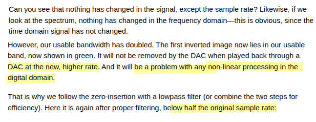
Inserting zeros changes nothing except what we consider the sample rate
Dan Boschen [https://dsp.stackexchange.com/a/32130/59253]
Bourdopoulos, G. I. (2003). Delta-Sigma modulators : modeling, design and applications. Imperial College Press. [pdf]
DC Gain in IF
DC gain is used to compensate the ratio of sampling rate before and after upsample
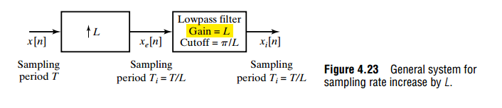
Given \[ X_e = X = \propto \frac{1}{T} = \frac{1}{L\cdot T_i} \] Then, the lowpass filter (ZOH, FOH .etc) gain shall be \(L\)
Employ definition of DTFT, \(X(e^{j\hat{\omega}}) =\sum_{n=-\infty}^{+\infty}x[n]e^{-j\hat{\omega} n}\), and set \(\hat{\omega} = 0\) \[ X(e^{j0}) = \sum_{n=-\infty}^{+\infty}x[n] \] That is, \(\sum_{n=-\infty}^{+\infty}x[n] = \sum_{n=-\infty}^{+\infty}x_e[n]\), so \[ \overline{x_e[n]} = \frac{1}{L} \overline{x[n]} \] It also indicate that dc gain of upsampling is \(1/L\)
Zero-Order Hold (ZOH)
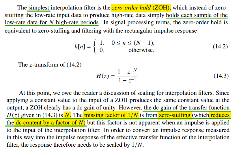
dc gain = \(N\)
First-Order Hold (FOH)
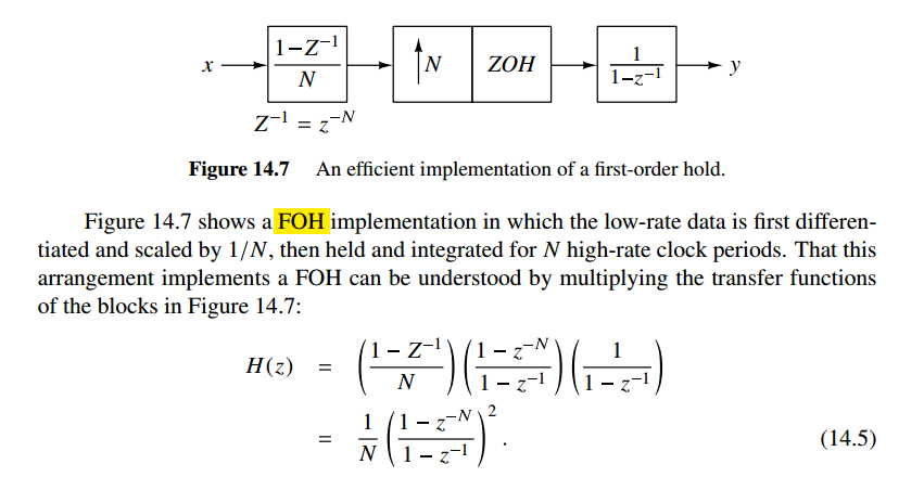
dc gain = \(N\)
Accumulate-and-dump (AAD) decimator
accumulating the input for \(N\) cycles and then latching the result and resetting the integrator
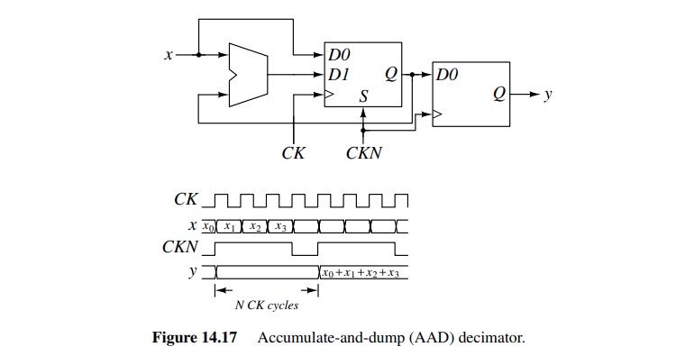
It adds up \(N\) succeeding input samples at rate \(1/T\) and delivers their sum in a single sample at the output. Therefore, the process comprises a filter (in the accumulation) and a down-sampler (in the dump)
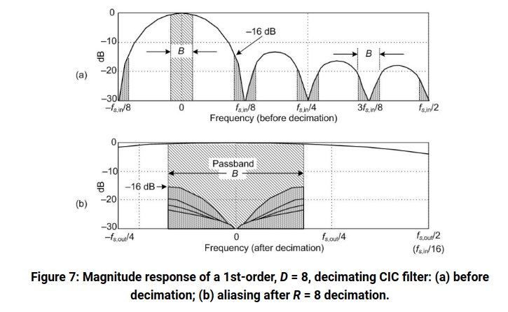
Cascaded Integrator-Comb (CIC) filter
Qasim Chaudhari, Cascaded Integrator Comb (CIC) Filters – A Staircase of DSP [https://wirelesspi.com/cascaded-integrator-comb-cic-filters-a-staircase-of-dsp/]
Tom Verbeure. An Intuitive Look at Moving Average and CIC Filters [https://tomverbeure.github.io/2020/09/30/Moving-Average-and-CIC-Filters.html]
—. Half-Band Filters, a Workhorse of Decimation Filters [https://tomverbeure.github.io/2020/12/15/Half-Band-Filters-A-Workhorse-of-Decimation-Filters.html]
—. Design of a Multi-Stage PDM to PCM Decimation Pipeline [https://tomverbeure.github.io/2020/12/20/Design-of-a-Multi-Stage-PDM-to-PCM-Decimation-Pipeline.html]
Arash Loloee, Ph.D. Exploring Decimation Filters [https://www.highfrequencyelectronics.com/Archives/Nov13/1311_HFE_decimationFilters.pdf]
Let's focus on decimation: if we decimate by a factor 4, we simply retain one output sample out of every 4 input samples.
In the example below, the downsampler at the right drops those 3 samples out of 4, and the output rate, \(y^\prime(n)\), is one fourth of the input rate \(x(n)\):
 \[\begin{align}
Y(z) &= X(z)\frac{1-z^{-4}}{1-z^{-1}} \\
Y^\prime(\xi) &= \frac{1}{4}Y(\xi^{1/4}) =
\frac{1}{4}X(\xi^{1/4})\frac{1-\xi^{-1}}{1-\xi^{-1/4}}
\end{align}\]
\[\begin{align}
Y(z) &= X(z)\frac{1-z^{-4}}{1-z^{-1}} \\
Y^\prime(\xi) &= \frac{1}{4}Y(\xi^{1/4}) =
\frac{1}{4}X(\xi^{1/4})\frac{1-\xi^{-1}}{1-\xi^{-1/4}}
\end{align}\]
with \(z=e^{j\Omega/f_s}\) and \(\xi =z^4\), we have \[ Y^\prime(z) = \frac{1}{4}X(z)\frac{1-z^{-4}}{1-z^{-1}} \]
But if we're going to be throwing away 75% of the calculated values, can't we just move the downsampler from the end of the pipeline to somewhere in the middle? Right between the integrator stage and the comb stage? That answer is yes, but to keep the math working, we also need to divide the number of delay elements in the comb stage by the decimation rate:

\[\begin{align} A(z) &= X(z)\frac{1}{1-z^{-1}} \\ A^\prime(\xi) &= \frac{1}{4}A(\xi^{1/4}) = \frac{1}{4}X(\xi^{1/4})\frac{1}{1-\xi^{-1/4}} \\ Y^\prime(\xi) &= A^\prime(\xi) (1-\xi^{-1}) = \frac{1}{4}X(\xi^{1/4})\frac{1-\xi^{-1}}{1-\xi^{-1/4}} \end{align}\]
with \(z=e^{j\Omega/f_s}\) and \(\xi =z^4\), we have \[ Y^\prime(z) = \frac{1}{4}X(z)\frac{1-z^{-4}}{1-z^{-1}} \]
And we can do this just the same with cascaded sections (without downsampler or updampler) where integrators and combs have been grouped
- for decimation, the integrators come first and the combs second with the downsampler in between
- For interpolation, the reverse is true
- the incoming sample rate is fraction of the outgoing sample rate, the combs must come first and the interpolators second


reference
Pavan, Shanthi, Richard Schreier, and Gabor Temes. (2016) 2016. Understanding Delta-Sigma Data Converters. 2nd ed. Wiley.
K. Hosseini and M. P. Kennedy, Minimizing Spurious Tones in Digital Delta-Sigma Modulators (Analog Circuits and Signal Processing). New York, NY, USA: Springer, 2011.
Neil Robertson, Model a Sigma-Delta DAC Plus RC Filter [https://www.dsprelated.com/showarticle/1642.php]
—, Modeling a Continuous-Time System with Matlab [https://www.dsprelated.com/showarticle/1055.php]
—, Modeling Anti-Alias Filters [https://www.dsprelated.com/showarticle/1418.php]
—, DAC Zero-Order Hold Models [https://www.dsprelated.com/showarticle/1627.php]
—, “A Simplified Matlab Function for Power Spectral Density”, DSPRelated.com, March, 2020, [https://www.dsprelated.com/showarticle/1333.php]
Ahmed Shahein (2026). MSD Toolbox (https://github.com/ahmedshahein/MSDTOOLBOX), GitHub. Retrieved April 25, 2026.
—, Multi-Decimation Stage Filtering for Sigma Delta ADCs: Design and Optimization [https://www.dsprelated.com/showarticle/1037.php]
Rick Lyons. A Beginner's Guide To Cascaded Integrator-Comb (CIC) Filters [https://www.dsprelated.com/showarticle/1337.php]
—, Optimizing the Half-band Filters in Multistage Decimation and Interpolation [https://www.dsprelated.com/showarticle/903.php]
Venkatesh Srinivasan, ISSCC 2019 T5: Noise Shaping in Data Converters
Nan Sun,IEEE CAS 2020: Break the kT/C Noise Limit [https://www.facebook.com/ieeecas/videos/break-the-ktc-noise-limit/322899188976197/]
Yun-Shiang Shu, ISSCC 2022 T3: Noise-Shaping SAR ADCs
Xiyuan Tang, CICC 2025 ES2-1: Noise-Shaping SAR ADCs - From Fundamentals to Recent Advances