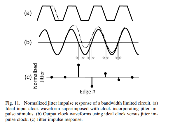
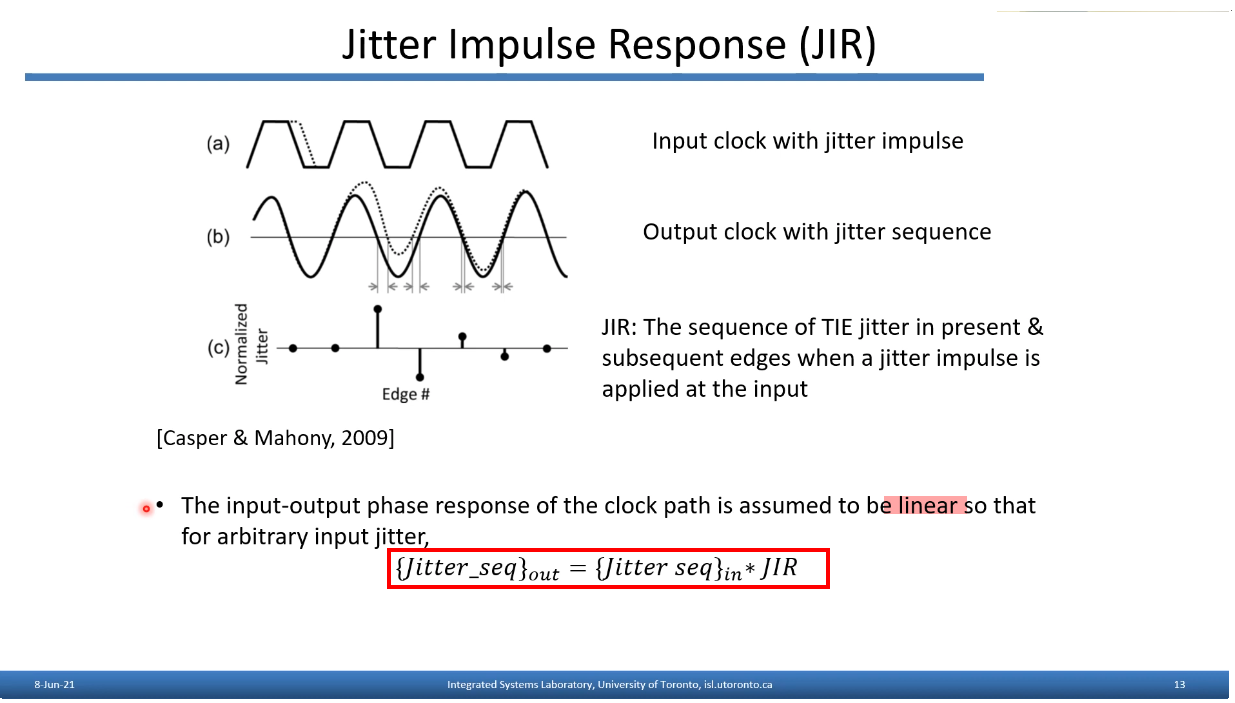
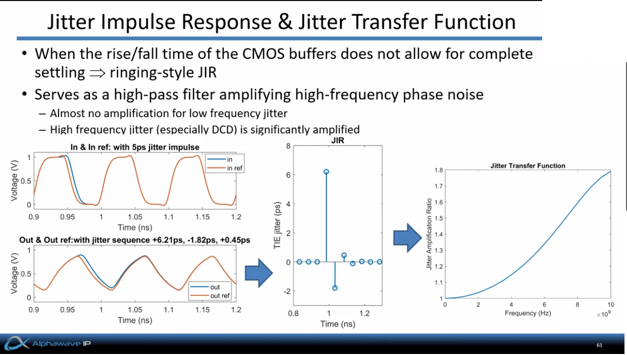
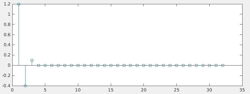
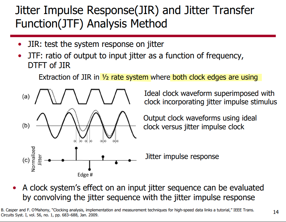
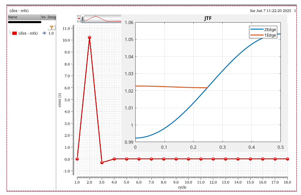
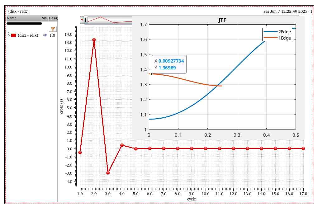
discrete time jitter impulse response
(normalized to the input jitter stimulus similar to the procedure used
to represent a conventional system impulse response)
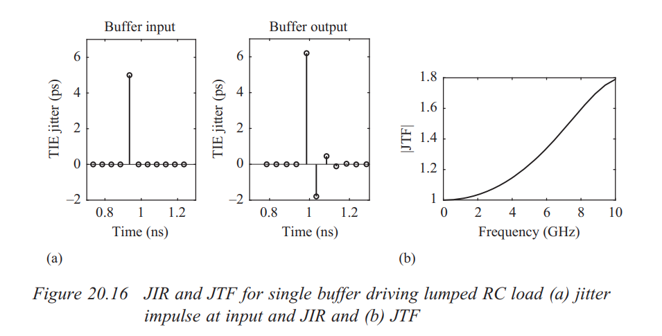
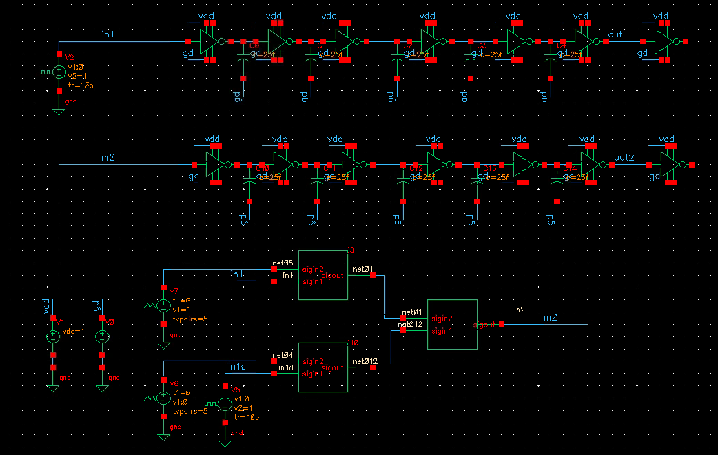
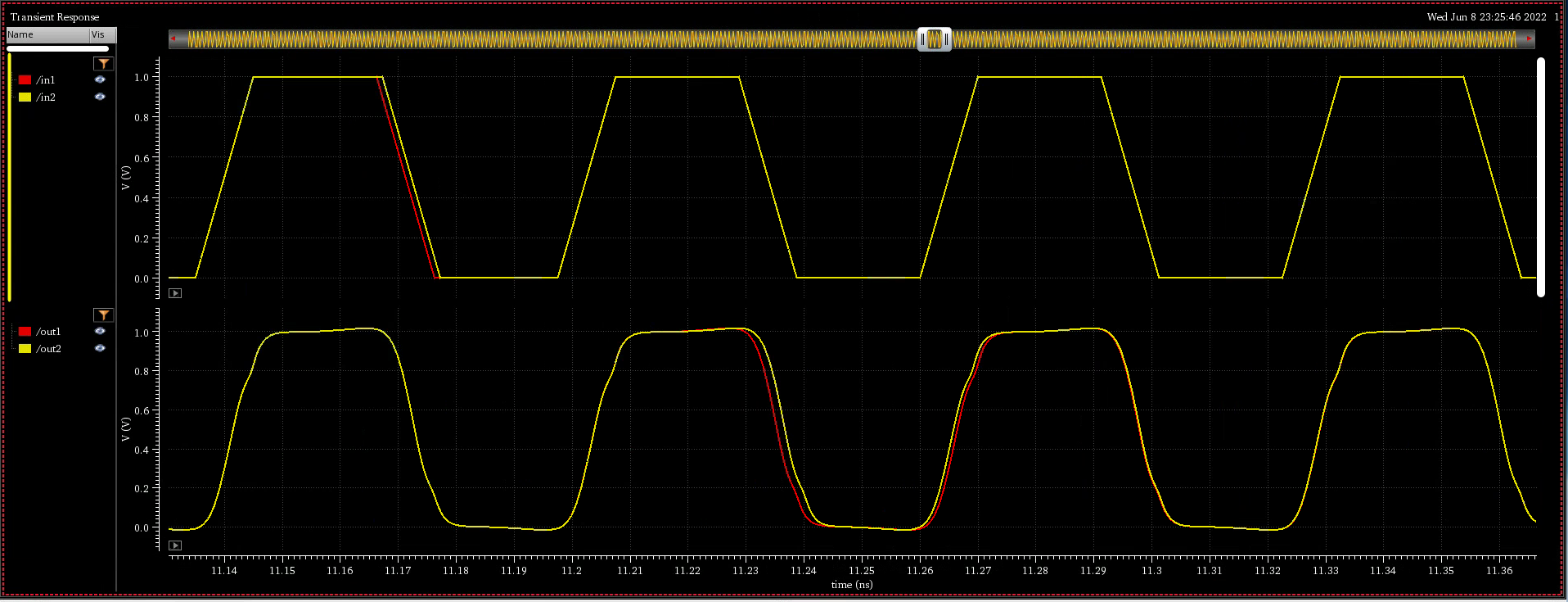
When impulsive jitter is injected into clock distribution circuits
(i.e., a small incremental time delay or advance applied to an
individual clock edge), it results in jitter in
multiple subsequent edges in the output clock
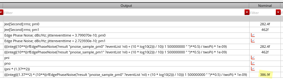
transient noise and
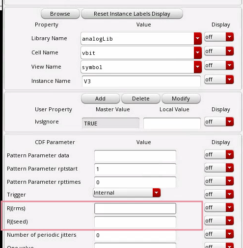
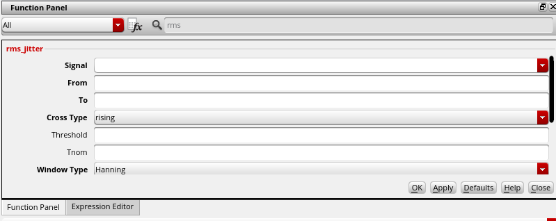
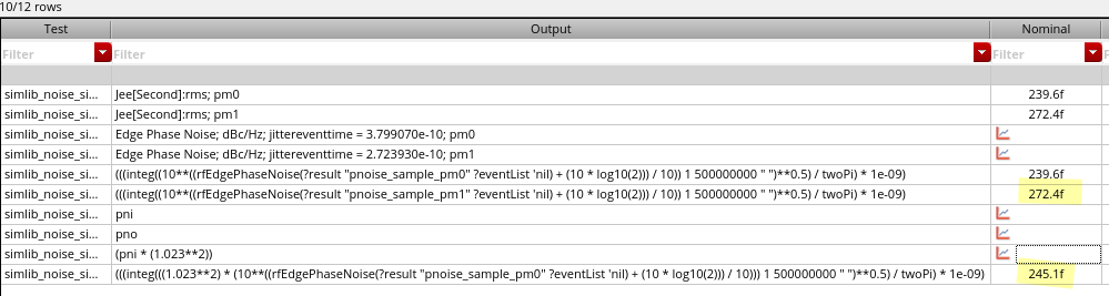
rms_jitter function
RJ(rms): single Edge or Both Edge?
RJ(seed): what is it?
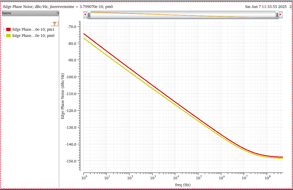
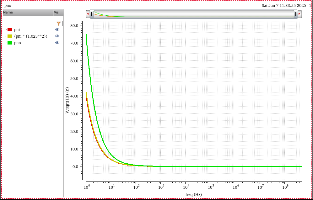
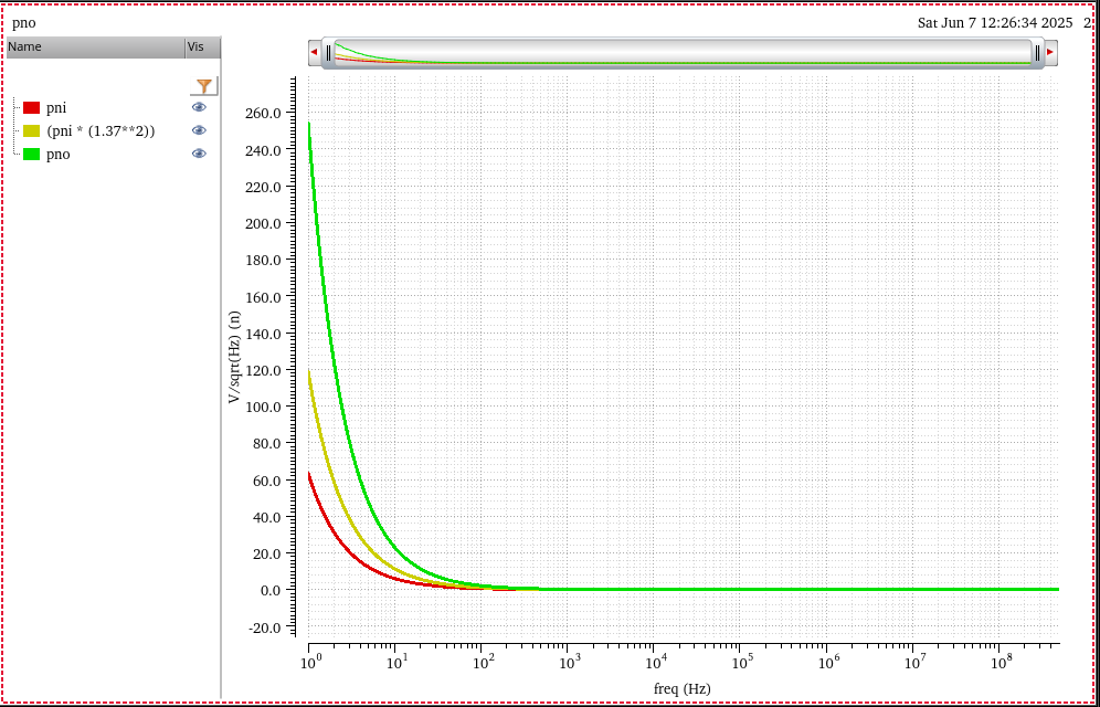
phase noise method
Directly compare the input phase noise and output phase noise, the
input waveform maybe is the PLL output or other clock distribution end
point
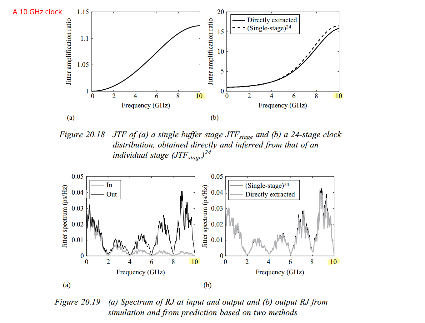
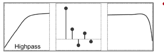
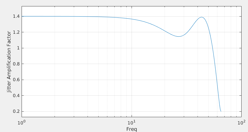
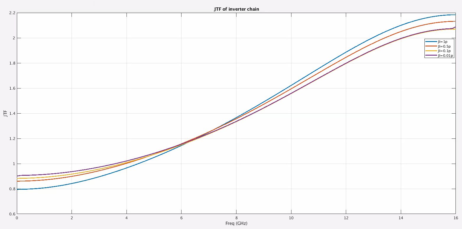
Jitter Impulse
Response & Jitter Transfer Function
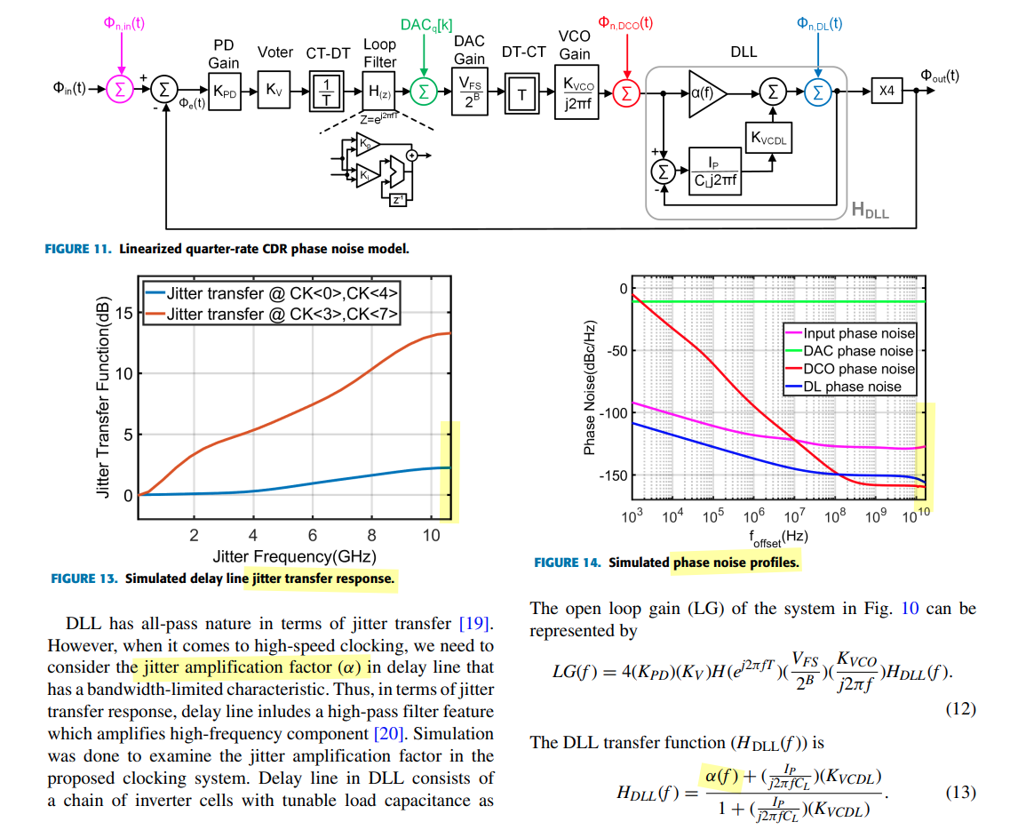
Four major noise sources are included in the modeling: Input noise,
DAC quantization noise (DAC QN), DCO random noise (DCO RN), and delay
line random noise (DL RN).
Rhee, W. (2020). Phase-locked frequency generation and clocking :
architectures and circuits for modern wireless and wireline
systems. The Institution of Engineering and TechnologyMathuranathan
Viswanathan, Digital Modulations using Matlab : Build Simulation Models
from Scratch
Tony Chan Carusone, University of Toronto, Canada, 2022 CICC
Educational Sessions "Architectural Considerations in 100+ Gbps Wireline
Transceivers"
Ganesh Balamurugan and Naresh Shanbhag, "Modeling and mitigation of
jitter in multiGbps source-synchronous I/O links," Proceedings 21st
International Conference on Computer Design, San Jose, CA, USA,
2003, pp. 254-260, doi: 10.1109/ICCD.2003 [https://shanbhag.ece.illinois.edu/publications/ganesh-ICCD2203.pdf]
Balamurugan, G. & Casper, Bryan & Jaussi, James &
Mansuri, Mozhgan & O'Mahony, Frank & Kennedy, Joseph. (2009).
Modeling and Analysis of High-Speed I/O Links. Advanced Packaging, IEEE
Transactions on. [https://sci-hub.se/10.1109/TADVP.2008.2011366]
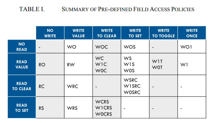
whether a register field can be read or written depends on both the
field's configured access policy and the register's rights in the map
being used to access the field
If a back-door access path is used, the effect of writing the
register through a physical access is mimicked. For example,
read-only bits in the registers will
not be written.
The mirrored value will be updated using the
uvm_reg::predict() method.
If a back-door access path is used, the effect of reading the
register through a physical access is mimicked. For example,
clear-on-read bits in the registers will be set to
zero.
The mirrored value will be updated using the
uvm_reg::predict() method.
Sample the value in the DUT register corresponding to this
abstraction class instance using a back-door access.
The register value is sampled, not modified.
Uses the HDL path for the design abstraction specified by
kind.
The mirrored value will be updated using the
uvm_reg::predict() method.
Read the register and optionally compared the readback
value with the current mirrored value if
check is UVM_CHECK.
The mirrored value will be updated using the
uvm_reg::predict() method based on the readback
value.
The mirroring can be performed using the physical interfaces
(frontdoor) or uvm_reg::peek() (backdoor).
If the register contains write-only fields,
their content is mirrored and optionally checked only if a
UVM_BACKDOOR access path is used to read the
register.
Write this register if the DUT register is out-of-date with the
desired/mirrored value in the abstraction class, as determined by the
uvm_reg::needs_update() method.
The update can be performed using the using the physical interfaces
(frontdoor) or uvm_reg::poke() (backdoor) access.
functionbit uvm_reg::needs_update(); needs_update = 0; foreach (m_fields[i]) begin if (m_fields[i].needs_update()) begin return1; end end endfunction: needs_update
// Concatenate the write-to-update values from each field // Fields are stored in LSB or MSB order upd = 0; foreach (m_fields[i]) upd |= m_fields[i].XupdateX() << m_fields[i].get_lsb_pos();
Update the mirrored and desired value for this
register.
Predict the mirror (and desired) value of the fields in the register
based on the specified observed value on a specified
address map, or based on a calculated value.
if (rw.status ==UVM_IS_OK ) rw.status = UVM_IS_OK;
if (m_is_busy && kind == UVM_PREDICT_DIRECT) begin `uvm_warning("RegModel", {"Trying to predict value of register '", get_full_name(),"' while it is being accessed"}) rw.status = UVM_NOT_OK; return; end
foreach (m_fields[i]) begin rw.value[0] = (reg_value >> m_fields[i].get_lsb_pos()) & ((1 << m_fields[i].get_n_bits())-1); m_fields[i].do_predict(rw, kind, be>>(m_fields[i].get_lsb_pos()/8)); end
UVM_PREDICT_DIRECT: begin if (m_parent.is_busy()) begin `uvm_warning("RegModel", {"Trying to predict value of field '", get_name(),"' while register '",m_parent.get_full_name(), "' is being accessed"}) rw.status = UVM_NOT_OK; end end endcase
// update the mirror with predicted value m_mirrored = field_val; m_desired = field_val; this.value = field_val;
Resetting a register model sets the mirror to the reset value
specified in the model
uvm_reg::reset
1 2 3 4 5 6 7 8 9 10
functionvoid uvm_reg::reset(string kind = "HARD"); foreach (m_fields[i]) m_fields[i].reset(kind); // Put back a key in the semaphore if it is checked out // in case a thread was killed during an operation void'(m_atomic.try_get(1)); m_atomic.put(1); m_process = null; Xset_busyX(0); endfunction: reset
m_mirrored = m_reset[kind]; m_desired = m_mirrored; value = m_mirrored;
if (kind == "HARD") m_written = 0;
endfunction: reset
uvm_reg_field::randomize
uvm_reg_field::pre_randomize()
Update the only publicly known property value with the
current desired value so it can be used as a state
variable should the rand_mode of the field be turned
off.
value is m_desired if
rand_mode is off.
1 2 3
functionvoid uvm_reg_field::pre_randomize(); value = m_desired; endfunction: pre_randomize
// Enum: uvm_predict_e // // How the mirror is to be updated // // UVM_PREDICT_DIRECT - Predicted value is as-is // UVM_PREDICT_READ - Predict based on the specified value having been read // UVM_PREDICT_WRITE - Predict based on the specified value having been written // typedefenum { UVM_PREDICT_DIRECT, UVM_PREDICT_READ, UVM_PREDICT_WRITE } uvm_predict_e;
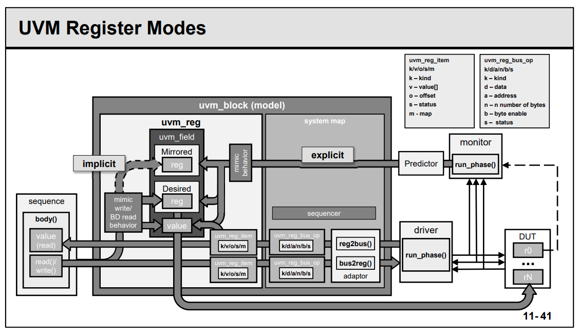
The generic register item is implemented as a struct in order to
minimise the amount of memory resource it uses. The struct is defined as
type uvm_reg_bus_op and this contains 6 fields:
Property
Type
Comment/Description
addr
uvm_reg_addr_t
Address field, defaults to 64 bits
data
uvm_reg_data_t
Read or write data, defaults to 64 bits
kind
uvm_access_e
UVM_READ or UVM_WRITE
n_bits
unsigned int
Number of bits being transferred
byte_en
uvm_reg_byte_en_t
Byte enable
status
uvm_status_e
UVM_IS_OK, UVM_IS_X, UVM_NOT_OK
1 2 3 4 5 6 7 8 9
typedefstruct { uvm_access_e kind; // Kind of access: READ or WRITE. uvm_reg_addr_t addr; // The bus address. uvm_reg_data_t data; // The data to write. // The number of bits of <uvm_reg_item::value> being transferred by this transaction. int n_bits; uvm_reg_byte_en_t byte_en; // Enables for the byte lanes on the bus. uvm_status_e status; // The result of the transaction: UVM_IS_OK, UVM_HAS_X, UVM_NOT_OK. } uvm_reg_bus_op;
The register class contains a build method which is used
to create and configure the
fields.
this build method is not called by the UVM
build_phase, since the register is an
uvm_object rather than an uvm_component
1 2 3 4 5 6
// // uvm_reg constructor prototype: // functionnew (string name="", // Register name intunsigned n_bits, // Register width in bits int has_coverage); // Coverage model supported by the register
As shown above, Register width is 32 same with the
bus width, lower 14 bit is configured.
RTL
1 2
`define SPI_CTRL_BIT_NB 14 reg [`SPI_CTRL_BIT_NB-1:0] ctrl; // Control and status register
Register Maps
Two purpose of the register map
provide information on the offset of the registers, memories and/or
register blocks
identify bus agent based sequences to be executed ???
There can be several register maps within a block, each one can
specify a different address map and a different
target bus agent
register map has to be created which the register
block using the create_map method
1 2 3 4 5 6 7 8 9 10 11 12 13
// // Prototype for the create_map method // function uvm_reg_map create_map(string name, // Name of the map handle uvm_reg_addr_t base_addr, // The maps base address intunsigned n_bytes, // Map access width in bytes uvm_endianness_e endian, // The endianess of the map bit byte_addressing=1); // Whether byte_addressing is supported // // Example: // AHB_map = create_map("AHB_map", 'h0, 4, UVM_LITTLE_ENDIAN);
The n_bytes parameter is the word size (bus
width) of the bus to which the map is associated. If a register's width
exceeds the bus width, more than one bus access is needed to read and
write that register over that bus.
he byte_addressing argument affects how the address is
incremented in these consecutive accesses. For example, if
n_bytes=4 and byte_addressing=0, then an access to a
register that is 64-bits wide and at offset 0 will result in two bus
accesses at addresses 0 and 1. With byte_addressing=1, that
same access will result in two bus accesses at addresses 0 and 4.
The default for byte_addressing is
1
The first map to be created within a register
block is assigned to the default_map member of the
register block
Register Adapter
uvm_reg_adapter
Methods
Description
reg2bus
Overload to convert generic register access items to target bus
agent sequence items
bus2reg
Overload to convert target bus sequence items to register model
items
Properties (Of type bit)
Description
supports_byte_enable
Set to 1 if the target bus and the target bus agent supports byte
enables, else set to 0
provides_responses
Set to 1 if the target agent driver sends separate response
sequence_items that require response handling
The provides_responses bit should be set if the
agent driver returns a separate response item (i.e.
put(response), or item_done(response)) from
its request item
Prediction
the update, or prediction, of the register model content can occur
using one of three models
Auto Prediction
This mode of operation is the simplest to implement, but suffers from
the drawback that it can only keep the register model up to date with
the transfers that it initiates. If any other sequences
directly access the target sequencer to update register content, or if
there are register accesses from other DUT interfaces, then the register
model will not be updated.
// Gets the auto-predict mode setting for this map. functionbit uvm_reg_map::get_auto_predict(); return m_auto_predict; endfunction
// Function: set_auto_predict
//
// Sets the auto-predict mode for his map.
//
// When on is TRUE,
// the register model will automatically update its
mirror (what it thinks should be in the DUT)
immediately after any bus read or write operation via this map.
Before a uvm_reg::write
// or uvm_reg::read operation returns, the register's
uvm_reg::predict method is called to update
the mirrored value in the register.
//
// When on is FALSE, bus reads and writes via
this map do not
// automatically update the mirror. For real-time updates to the
mirror
// in this mode, you connect a uvm_reg_predictor
instance to the bus
// monitor. The predictor takes observed bus transactions from
the
// bus monitor, looks up the associated uvm_reg register
given
// the address, then calls that register's
uvm_reg::predict method.
// While more complex, this mode will capture all register
read/write
// activity, including that not directly descendant from calls to
// uvm_reg::write and uvm_reg::read.
//
// By default, auto-prediction is turned off.
//
The register model content is updated based on the register accesses
it initiates
Explicit Prediction
(Recommended Approach)
Explicit prediction is the default mode of
prediction
The register model content is updated via the predictor
component based on all observed bus transactions, ensuring that
register accesses made without the register model are mirrored
correctly. The predictor looks up the accessed register by address then
calls its predict() method
if (m_is_busy && kind == UVM_PREDICT_DIRECT) begin `uvm_warning("RegModel", {"Trying to predict value of register '", get_full_name(),"' while it is being accessed"}) rw.status = UVM_NOT_OK; return; end foreach (m_fields[i]) begin rw.value[0] = (reg_value >> m_fields[i].get_lsb_pos()) & ((1 << m_fields[i].get_n_bits())-1); m_fields[i].do_predict(rw, kind, be>>(m_fields[i].get_lsb_pos()/8)); end
UVM_PREDICT_DIRECT: begin if (m_parent.is_busy()) begin `uvm_warning("RegModel", {"Trying to predict value of field '", get_name(),"' while register '",m_parent.get_full_name(), "' is being accessed"}) rw.status = UVM_NOT_OK; end end endcase
// update the mirror with predicted value m_mirrored = field_val; m_desired = field_val; this.value = field_val;
endfunction: do_predict
uvm_access_e
1 2 3 4 5 6 7 8 9 10 11 12 13
// Enum: uvm_access_e // // Type of operation begin performed // // UVM_READ - Read operation // UVM_WRITE - Write operation // typedefenum { UVM_READ, UVM_WRITE, UVM_BURST_READ, UVM_BURST_WRITE } uvm_access_e;
uvm_predict_e
1 2 3 4 5 6 7 8 9 10 11 12 13
// Enum: uvm_predict_e // // How the mirror is to be updated // // UVM_PREDICT_DIRECT - Predicted value is as-is // UVM_PREDICT_READ - Predict based on the specified value having been read // UVM_PREDICT_WRITE - Predict based on the specified value having been written // typedefenum { UVM_PREDICT_DIRECT, UVM_PREDICT_READ, UVM_PREDICT_WRITE } uvm_predict_e;
uvm_path_e
1 2 3 4 5 6 7 8 9 10 11 12 13 14 15 16
// Enum: uvm_path_e // // Path used for register operation // // UVM_FRONTDOOR - Use the front door // UVM_BACKDOOR - Use the back door // UVM_PREDICT - Operation derived from observations by a bus monitor via // the <uvm_reg_predictor> class. // UVM_DEFAULT_PATH - Operation specified by the context // typedefenum { UVM_FRONTDOOR, UVM_BACKDOOR, UVM_PREDICT, UVM_DEFAULT_PATH } uvm_path_e;
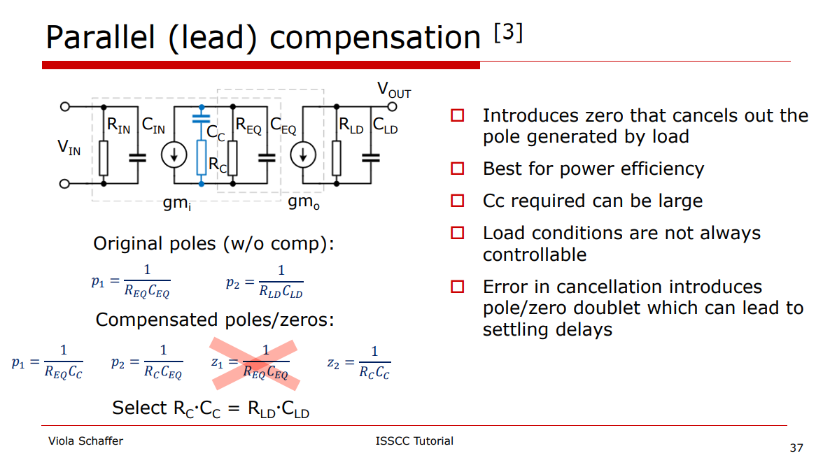
Parallel Compensation is also known as Lead
Compensation, Pole-Zero Compensation
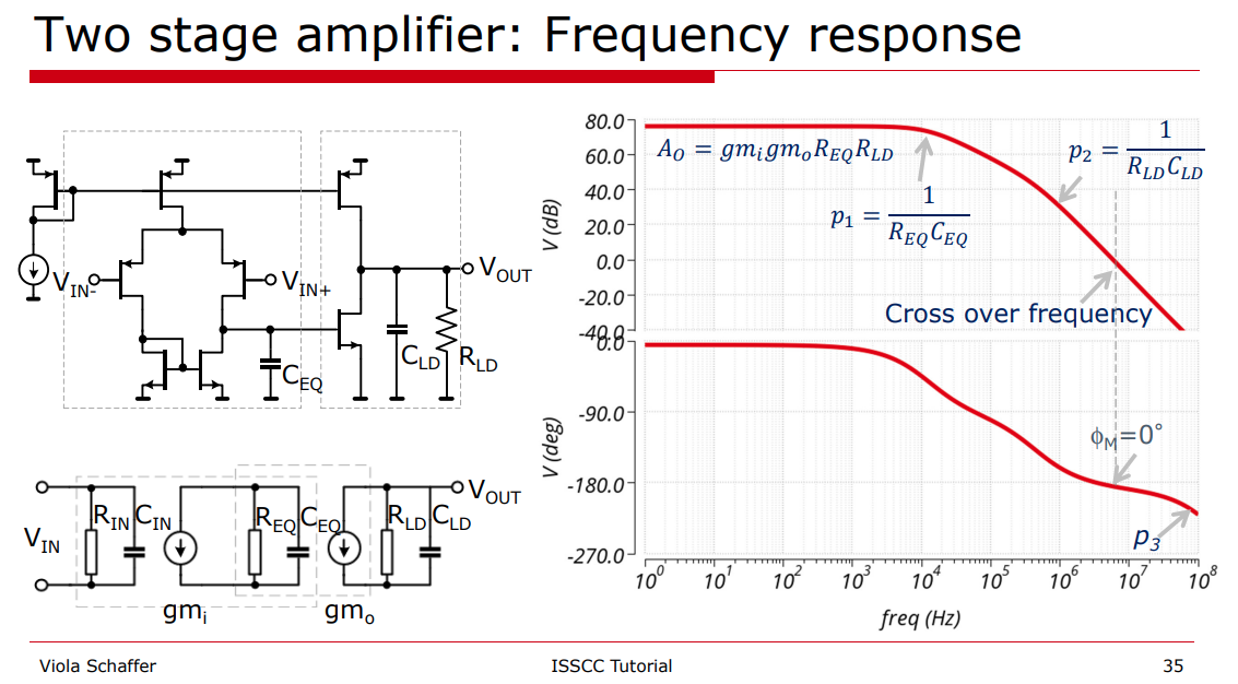
Note: The dominant pole is at output of the first
stage, i.e. \(\frac{1}{R_{EQ}C_{EQ}}\).
Pole and Zero in transfer
function
Design with operational amplifiers and analog integrated circuits /
Sergio Franco, San Francisco State University. – Fourth edition
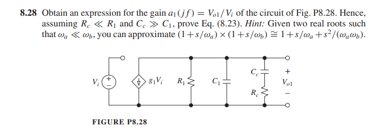
\[
Y = \frac{1}{R_1} + sC_1+\frac{1}{R_c+1/SC_c}
\]
\[\begin{align}
Z &= \frac{1}{\frac{1}{R_1} + sC_1+\frac{1}{R_c+1/SC_c}} \\
&= \frac{R_1(1+sR_cC_c)}{s^2R_1C_1R_cC_c+s(R_1C_c+R_1C_1+R_cC_c)+1}
\end{align}\] If \(p_{1c} \ll
p_{3c}\), two real roots can be found \[\begin{align}
p_{1c} &= \frac{1}{R_1C_c+R_1C_1+R_cC_c} \\
p_{3c} &= \frac{R_1C_c+R_1C_1+R_cC_c}{R_1C_1R_cC_c}
\end{align}\]
The additional zero is \[
z_c = \frac{1}{R_cC_c}
\] Given \(R_c \ll R\) and \(C_c \gg C\)\[\begin{align}
p_{1c} &\simeq \frac{1}{R_1(C_c+C_1)} \simeq \frac{1}{R_1C_c}\\
p_{3c} &= \frac{1}{R_cC_1}+\frac{1}{R_cC_c}+\frac{1}{R_1C_1} \simeq
\frac{1}{R_cC_1}
\end{align}\]
The output pole is unchanged, which is \[
p_2 = \frac{1}{R_LC_L}
\] We usually cancel\(p_2\) with \(z_c\), i.e. \[
R_cC_c=R_LC_L
\]
Phase margin
unity-gain frequency \(\omega_t\)\[
\omega_t = A_\text{DC}\cdot P_{1c} =\frac{g_{m1}g_{m2}R_L}{C_c}
\]
PM=45\(^o\)\[
p_{3c} = \omega_t
\] Then, \(C_c\) and \(R_c\) can be obtained
for the unity-gain frequency \(\omega_t\) we find \[
\omega_t = \sqrt{\frac{1}{2}\cdot \frac{g_{m1}g_{m2}}{C_1C_L}}
\] The parallel compensation shows a remarkably good result. The
new 0 dB frequency lies only a factor \(\sqrt{2}\) lower than the theoretical
maximum
To increase \(\phi_m\), we need to
raise\(C_c\) a bit
while lowering\(R_c\)
in proportion in order to maintain pole-zero cancellation. This causes
\(p_{1c}\) and \(p_{3c}\) to split a bit further apart.
ri = 2; % PM=45: 1; PM=60: 2 Rc = (R/C/fnd/2/pi/ri/Adc)^0.5; % compensation resistor Cc = (ri*Adc*C/fnd/2/pi/R)^0.5; % compensation capacitor
wzc = 1/2/pi/Rc/Cc; % zero frequency
reference
Viola Schäffer, Designing Amplifiers for Stability, ISSCC 2021
Tutorials
R.Eschauzier "Wide Bandwidth Low Power Operational Amplifiers", Delft
University Press, 1994.
Gene F. Franklin, J. David Powell, and Abbas Emami-Naeini. 2018.
Feedback Control of Dynamic Systems (8th Edition) (8th. ed.). Pearson.
6.7 Compensation
Application Note AN-1286 Compensation for the LM3478 Boost
Controller
A conventional inverter-based ring oscillator consists of a single
loop of an odd number of inverters. While compact, easy
to design and tunable over a wide frequency range, this oscillator
suffers from several limitations.
it is not possible to increase the number of phases while
maintaining the same oscillation frequency since the frequency is
inversely proportional to the number of inverters in the loop. In other
words, the time resolution of the oscillator is limited to one inverter
delay and cannot be improved below this limit.
the number of phases that can be obtained from this oscillator is
limited to odd values. Otherwise, if an even number of
inverters is used, the circuit remains in a latched state and
does not oscillate.
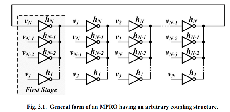
To overcome the limitations of conventional ring oscillators,
multi-paths ring oscillator (MPRO) is proposed. Each phase can be driven
by two or more inverters, or multi-paths instead of having each
phase in oscillator driven by a single inverter, or single
path.
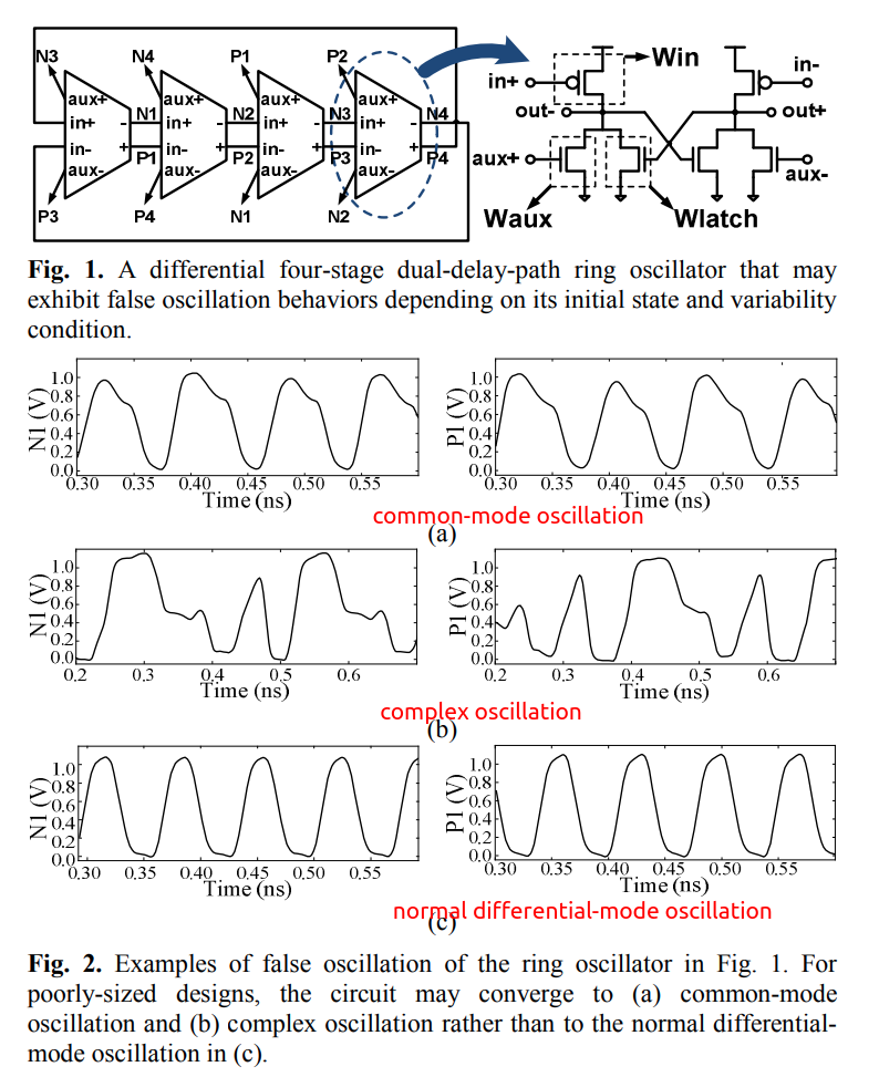
One thing that makes the MPRO design problem even more complicated is
its property of having multiple possible oscillation
modes. Without a clear understanding of what makes one of these
modes dominant, it is very likely that a designer might end-up having an
oscillator that can start-up each time in a different oscillation mode
depending on the initial state of the oscillator.
In practive, the oscillator starts first from a linear mode of
operation where all the buffers are indeed acting as linear
transconductors. All oscillation modes that have mode gains, \(a_n\), lower than the actual dc gain of the
inverter, \(a_0\), start to grow.
As the oscillation amplitude grows, the effective gain of the
inverter drops due to nonlinearity. Consequently, modes with higher
mode gain die out and only the mode that requires the minimum gain
continues to oscillate and hence is the dominant mode.
The dominant mode is dependent only on the relative sizing vector
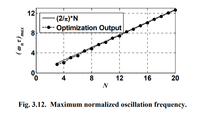
maximum oscillation
frequency
The oscillation frequency of the dominant mode of any MPRO having any
arbitrary coupling structure and number of phases is \[
f_{n^*} = \frac {1}{2\pi}\frac {(a_0-1) \cdot \sum_{i=1}^{N}x_isin\left
( \frac {2\pi n^*(i-1)}{N} \right)}{(a_0\tau _p - \tau _o)\cdot
\sum_{i=1}^{N}-x_icos\left( \frac{2\pi n^*(i-1)}{N}+(\tau _o - \tau _p)
\right)}
\]
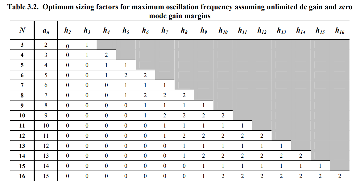
A linear increase in the maximum possible normalized
oscillation frequency as the number of stages increases provided
that the dc gain of the buffer sufficient to provide the required
amplification
assuming unlimited dc gain and zero mode gain margins
mode stability
A common problem in MPRO design is the stability of the dominant
oscillation mode. Mode stability refers to whether the MPRO always
oscillates at the same mode regardless of the initial conditions of the
oscillator. This problem is especially pronounced for MPROs with a large
number of phases. This is due to the existence of many modes and the
very small differences in the value of the mode gain of adjacent modes
if the MPRO is not well designed.
In general, when the mode gain difference between two modes is small,
the oscillator can operate in either one depending on initial
conditions.
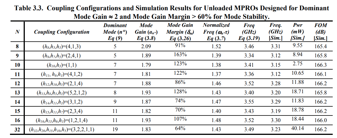
coupling
configurations and simulation results
Abou-El-Sonoun, A. A. (2012). High Frequency Multiphase Clock
Generation Using Multipath Oscillators and Applications. UCLA.
ProQuest ID: AbouElSonoun_ucla_0031D_10684. Merritt ID:
ark:/13030/m57p9288. Retrieved from
https://escholarship.org/uc/item/75g8j8jt
frequency stability
A problem associated with the design of MPROs is the existence of
different possible modes of oscillation. Each of these modes is
characterized by a different frequency, phase shift and phase noise.
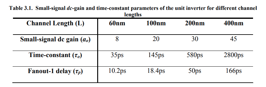
Linear delay-stage model
(mode gain)
mode gain is based on the linear model, independent
of process but depends on coupling structure (coupling configuration,
size ratio).
The inverting buffer modeled as a linear transconductor. The
input-output relationship of a single buffer scaled by \(h_i\) and driving the input capacitance of
a similar buffer can be expressed as \[\begin{align}
h_ig_mv_{in}(t) + h_ig_oV_{out}(t)+h_iC_g\frac {dV_{out}(t)}{dt} &=
0 \\
a_nV_{in}(t)+V_{out}(t)+\tau \frac {V_{out}(t)}{dt} &= 0
\end{align}\] where \(g_m\) is
the transconductance, \(g_o\) is the
output conductance, \(C_g\) is the
buffer input capacitance which also acts as the load capacitance for the
driving buffer, and \(a_n = \frac
{g_m}{g_o}\) is the linear dc gain of the
buffer, and \(\tau=\frac {C_g}{g_o}\)
is a time constant.
Similarly, \(V_1\), the output of
the first stage in MPRO can be expressed \[
\sum_{i=1}^{N}h_ig_mV_i(t)+\sum_{i=1}^{N}h_ig_oV_i(t)+\sum_{i=1}^{N}h_iC_g\frac
{dV_it(t)}{dt} = 0
\] Defining the fractional sizing factors and the total sizing
factor as \(x_i=\frac{h_i}{H}\) and
\(H=\sum_{i=1}^{N}h_i\)\[
a_n\sum_{i=1}^{N}x_iV_i(t) + V_1(t)+\tau\frac {dV_i(t)}{dt} = 0
\] where \(a_n = \frac
{g_m}{g_o}\) and \(\tau=\frac
{C_g}{g_o}\) are same dc gain and time constant defined
previously
Since the total phase shift around the loop should be multiples of
\(2\pi\), the oscillation waveform at
the ith node can be expressed as \[
V_i(t) = V_o \cos(\omega_nt-\Delta \varphi \cdot i)
\] where \(\omega_n\) is the
oscillation frequency and \(\Delta \varphi =
\frac {2\pi n}{N}\), \(N\) is
the number of stages in the oscillator and \(n\) can take values between \(0\) and \(N-1\)
Plug \(V_i(t)\) into differential
equation, we get \[
a_n\sum_{i=1}^{N}x_i\cos(\omega_n t-\frac{2\pi n}{N}i)+\cos(\omega_n
t-\frac{2\pi n}{N}) - \omega_n \tau \sin(\omega_n t-\frac{2\pi n}{N}) =
0
\] By equating the \(cos(\omega_n
t)\) and \(sin(\omega_n t)\)
terms of the above equation, we get expressions for the
oscillation frequency of the nth mode and the
minimum dc gain required for this mode to exist. we refer to
this gain as the mode gain\[\begin{align}
\omega_n\tau &= \frac {\sum_{i=1}^{N}x_i \cdot \sin(\frac{2\pi
n}{N}(i-1))}{-\sum_{i=1}^{N}x_i \cdot \cos(\frac{2\pi n}{N}(i-1))} \\
a_n &= \frac {1}{-\sum_{i=1}^{N}x_i \cdot \cos(\frac{2\pi
n}{N}(i-1))}
\end{align}\] where \(a_n\)
should be greater than \(0\) for a
existent mode
In practice, the oscillator starts first from a linear mode of
operation where all the buffers are indeed acting as linear
transconductors. All oscillation modes that have mode gains \(a_n\) lower than the actual dc gain of the
inverter \(a_o\) start to grow. As the
oscillation amplitude grows, the effective gain of the inverter drops
due to nonlinearity. Consequently, modes with higher mode gain die
out and only the mode that requires the minimum gain continues to
oscillate and hence is the dominant mode
A. A. Hafez and C. K. Yang, "Design and Optimization of Multipath
Ring Oscillators," in IEEE Transactions on Circuits and Systems I:
Regular Papers, vol. 58, no. 10, pp. 2332-2345, Oct. 2011, doi:
10.1109/TCSI.2011.2142810.
Simulation-based approach
GCHECK is an automated verification tool that
validate whether a ring oscillator always converges to the desired mode
of operation regardless of the initial conditions and
variability conditions. This is the first tool ever
reported to address the global convergence failures in presence of
variability. It has been shown that the tool can successfully validate a
number of coupled ring oscillator circuits with various global
convergence failure modes (e.g. no oscillation, false oscillation, and
even chaotic oscillation) with reasonable computational costs such as
running 1000-point Monte-Carlo simulations for 7~60 initial conditions
(maximum 4 hours).
The verification is performed using a predictive global
optimization algorithm that looks for a problematic initial
state from a discretized state space
despite the finite number of initial state
candidates considered and finite number of Monte-Carlo
samples to model variability, the proposed algorithm can verify
the oscillator to a prescribed confidence level
The observation that the responses of a circuit with nearby initial
conditions are strongly correlated with respect to common variability
conditions enables us to explore a discretized version
of the initial condition space instead of the continuous one.
the settling time increases as the initial state gets farther away
from the equilibrium state allowed us to use the settling time as a
guidance metric to find a problematic initial condition.
Selecting the Next Initial Condition Candidate to
Evaluate
To determine whether the algorithm should continue or terminate the
search for a new maximum, the algorithm estimates the probability of
finding a new initial condition with the longer settling
time, based on the information obtained with the
previously-evaluated initial conditions.
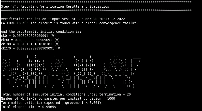
GCHECK EXAMPLE
1
python gcheck_osc.py input.scs
output log:
1 2 3 4 5 6 7 8
Step 1/4: Simulating the setting-time distribution with the reference initial condition ... Step 2/4: Simulating the setting-time distribution for randomly-selected initial probes ... Step 3/4: Searching for Problematic Initial Conditions ... Step 4/4: Reporting Verification Results and Statistics ...
T. Kim, D. -G. Song, S. Youn, J. Park, H. Park and J. Kim, "Verifying
start-up failures in coupled ring oscillators in presence of variability
using predictive global optimization," 2013 IEEE/ACM International
Conference on Computer-Aided Design (ICCAD), 2013, pp. 486-493, doi:
10.1109/ICCAD.2013.6691161.GCHECK: Global Convergence
Checker for Oscillators
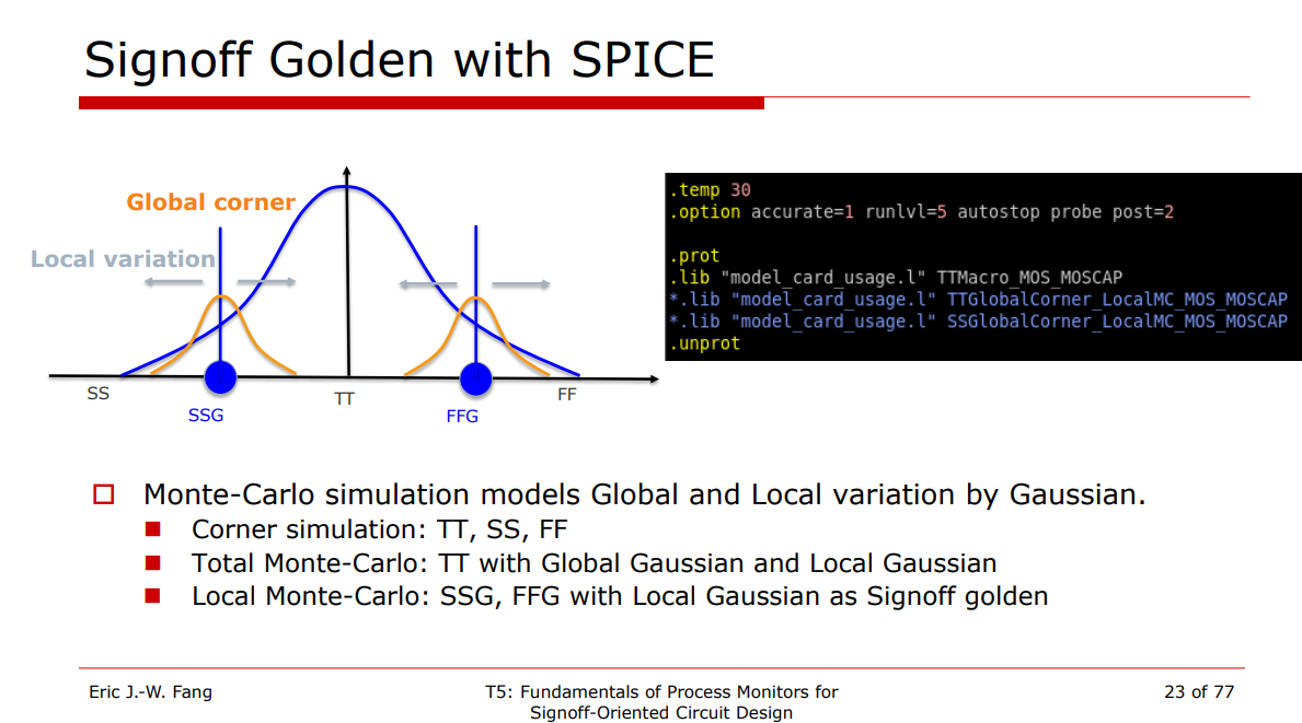
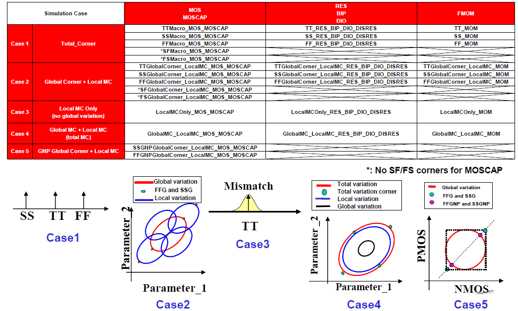
Local Monte-Carlo (SSG, FFG with Local Gaussian) as
Signoff golden
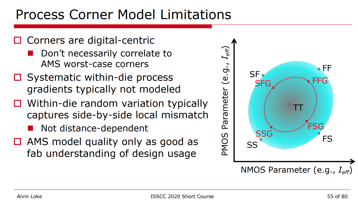
Process Corner Model
Limitations
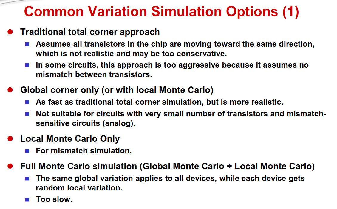
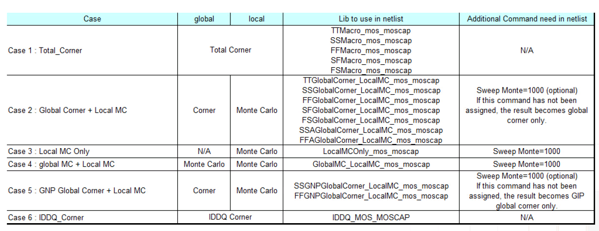
Variation section
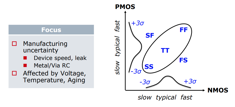
Total corner (TT/SS/FF/SF/FS)
E.g. TTMacro_MOS_MOS_MOSCAP
Global Corner (TTG/SSG/FFG/SFG/FSG) + Local MC
E.g. TTGlobalCorner_LocalMC_MOS_MOSCAP
Local MC
E.g. LocalMCOnly_MOS_MOSCAP
Global MC + Local MC (Total MC)
GlobalMC_LocalMC_MOS_MOSCAP
SSGNP, FFGNP:
When N/P global correlation is weak (R^2=0.15), the corner of N/PMOS
balance circuit (e.g. inverter) can be tightened (3sigma ->
2.5sgma) due to the cancellation between NMOS
and PMOS
SSGNP, FFGNP usually used in Digital STA
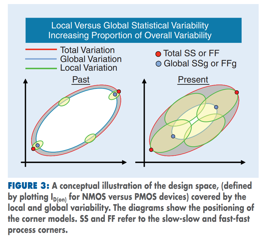
Global variation validation with global
corner
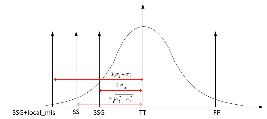
3-sigma of global MC simulation is aligned with
global corner
Total variation validation with total
corner
3-sigma of global MC + local MC (total) simulation
is aligned with total corner
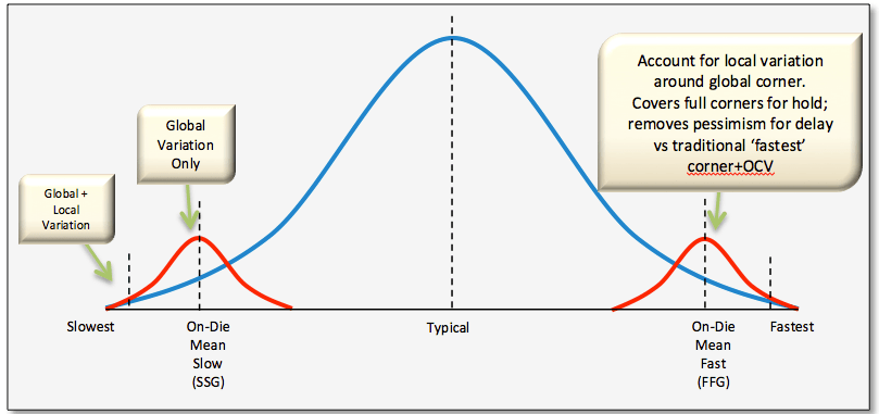
The "total corner" is representative of the maximum
device parameter variation including local device variation effects.
However, it is not a statistical corner.
The "global" corner is defined as the
"total" corner minus the impact of "local
variation"
Hence, if you were to examine simulation results for a parameter
using a "total" and "global" corner, you would find the range of
variation will be less with the "global" corner than with the "total"
corner.
The "global" corner is provided for use in statistical
simulations. Hence, when performing a Monte-Carlo simulation,
the "global" corner is selected - NOT the "total" corner.
Radojcic, Riko, Dan Perry and Mark Nakamoto. “Design for
manufacturability for fabless manufactuers.” IEEE Solid-State
Circuits Magazine 1 (2009): n. pag.
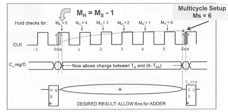
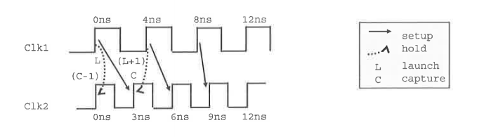
MH stands for Hold Multiplier, MS for Setup
Multiplier. The Setup multiplier counts up with increasing clock cycles,
the Hold Multiplier counts up with decreasing cycles. The origin (0) for
the Hold Multiplier is always at the Setup Multiplier - 1
position.
Reporting a
multicycle path with report_timing
1
report_timing -exceptions all -from *reg[26]/CP -to *reg/D
Timing Exceptions
If certain paths are not intended to operate
according to the default setup and hold behavior assumed by the
PrimeTime tool, you need to specify those paths as timing
exceptions. Otherwise, the tool might incorrectly report those paths as
having timing violations.
The PrimeTime tool lets you specify the following types of
exceptions:
False path – A path that is never sensitized due to the logic
configuration, expected data sequence, or operating mode.
Multicycle path – A path designed to take more than one clock cycle
from launch to capture.
Minimum or maximum delay path – A path that must meet a delay
constraint that you explicitly specify as a time value.
REF
PrimeTime® User Guide Version O-2018.06-SP4 Chapter 1: Introduction
to PrimeTime Overview of Static Timing Analysis - Timing Exceptions
Primary clocks should be created at input ports and output pins of
black boxes.
Never create clocks on hierarchy pins. Creating clocks on hierarchy
will cause problems when reading SDF. The net timing arc becomes
segmented at the hierarchy and PrimeTime will be unable to annotate the
net successfully.
generated clocks
Generated clocks are generally created for waveform modifications of
a primary clock (not including simple inversions). PrimeTime does not
simulate a design and thus will not derive internally
generated clocks automatically - these clocks must be created by the
user and applied as a constraint.
PrimeTime caculate source latency for generated clocks if primary
clock is propagated, otherwise its source latency is
zero.
functionvoid test_base::start_of_simulation_phase(uvm_phase phase); super.start_of_simulation_phase(phase); uvm_top.print_topology(); // Will not compile in UVM-1.2 factory.print(); // Will not compile in UVM-1.2 endfunction
Global handles uvm_top and factory in uvm_pkg have been removed in
UVM-1.2 and later
Mechanism in UVM-1.1 and
UVM-1.2
Call the get() method of the class to retrieve the
singleton handle.
1 2 3 4 5
functionvoid test_base::start_of_simulation_phase(uvm_phase phase); super.start_of_simulation_phase(phase); uvm_root::get().print_topology(); // Works in UVM-1.1 & UVM-1.2 uvm_factory::get().print(); // Works in UVM-1.1 & UVM-1.2 endfunction
uvm_coreservice_t is the uvm-1.2 mechanism for
accessing all the central UVM services such as
uvm_root,uvm_factory,
uvm_report_server, etc.
1
2
3
4
5
6
7
// Using the uvm_coreservice_t:
uvm_coreservice_t cs;
uvm_factory f;
uvm_root top;
cs = uvm_coreservice_t::get();
f = cs.get_factory();
top = cs.get_root();