Modeling and Simulation in SystemVerilog

Posted on 2024-08-18 Edited on 2024-09-22 In analog

Single-Pole Filter & Complex Conjugate Pole pair

Single-Pole Filter and Complex Conjugate Pole pair in Event-Driven PWL model

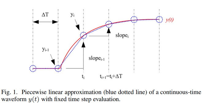
Real number modeling of analog circuits in hardware description languages (HDLs) has become more common as a part of mixed-signal SoC validation. Piecewise linear (PWL) waveform approximation represent analog signals and dynamically schedule the events for approximating the signal waveform to PWL segments with a well controlled error bound.

Definition of a piecewise liner (PWL) waveform using struct in Systemverilog

typedef struct {
    real y; // signal offset
    real slope; // signal slope
    real t0;	// time offset
} pwl; // pwl datatype

When to update piecewise model

model parameter update once new input come in
error is greater than user-define tolerance \(e_{tol}\), trigger by \(\Delta T\)

tolerance_error.drawio

Dynamic Time Step Control

When approximating a function \(y(t)\) to a piecewise linear segment for the interval \(t_0 \le t_0 + \Delta t\), the approximation error \(err\) is bounded by \[ \left| err \right| \le \frac{1}{8}\cdot \Delta t^2 \cdot \max(\left| \ddot{y(t)} \right|) \] Using Rolle's theorem for the interval \(t_0 \le t_0 + \Delta t\), the needed time step \(\Delta t\) is givend by \[ \Delta t(t=t_0) = \sqrt{\frac{8\cdot e_{tol}}{\max(\left| \ddot{y(t)} \right|)}} \]

Single-Pole Filter Model

The ramp input \(X(s)\), the single pole system Laplace s-domain \(H(s)\) and the output response \(Y(s)\), \[\begin{align} X(s) &= \frac{a}{s} +\frac{b}{s^2} \\ H(s) &= \frac{Y(s)}{X(s)} = \frac{1}{1+\frac{s}{\omega_{1}}} \\ Y(s) &= X(s) \cdot H(s) \end{align}\]

Time domain of ramp input shown as below \[ x(t) = a +b \cdot t \]

The output transfer function \[\begin{align} Y(s) &= X(s) \cdot H(s) \\ &= \frac{\omega_1}{\omega_1+s}\cdot X \end{align}\]

\[ Y\omega_1 + sY = \omega_1 X \]

its differential equation

\[ y(t) \cdot \omega_1+\frac{d y(t)}{dt} = \omega_1 \cdot x(t) \]

Laplace transfrom two side of the above equation, \(y_0\) is initial conditon of output, \(x_0=0\)

\[ Y\omega_1 + sY-y_0 = \omega_1 \cdot X \]

Solving \(Y(s)\) \[\begin{align} Y &= \frac{y_0}{\omega_1+s}+\frac{\omega_1}{\omega_1+s}\cdot X \\ &= \frac{y_0}{\omega_1+s}+\frac{\omega_1}{\omega_1+s}\cdot (\frac{a}{s}+\frac{b}{s^2}) \\ &= \frac{y_0}{\omega_1+s}+\frac{\omega_1}{\omega_1+s}\cdot \frac{a}{s}+\frac{\omega_1}{\omega_1+s}\cdot\frac{b}{s^2} \end{align}\]

inverse Laplace transform

\[ y(t) = y_0e^{-\omega_1t}+(a-a\cdot e^{-\omega_1t})+(b\cdot t-\frac{b}{\omega_1}+\frac{b}{\omega_1}\cdot e^{-\omega_1 t}) \]

step-1 transfer function in Laplace s-domain, which don't initial conditon and is only steady response.

step-2 differential equation

step-3 Laplace transform of \(Y(s)\), (the initial conditon of input \(X(s)\) is zero, that of \(Y(s)\) is explicit)

step-4 inverse Laplace transform, with the help of Laplace transform table or matlab syms and ilaplace function

\(y(t)\) has a continuous second derivative \(\ddot{y(t)}\) \[ \ddot{y(t)} =(-a+\frac{b}{\omega_1}+y_0)\cdot \omega_1^2\cdot e^{-\omega_1t} \] It's obvious \(\left| \ddot{y(t)} \right|\) is a decaying function and thus the maximum value is \(\left| \ddot{y(t_0)} \right|\) for the interval \(t_0 \le t_0 + \Delta t\). The time step \(\Delta t\) for the error tolerance \(e_{tol}\): \[ \Delta t(t=t_0) = \sqrt{\frac{8\cdot e_{tol}}{\left| \ddot{y(t_0)} \right|}} \]

Complex Conjugate Pole pair

\[ H(s) = \frac{r}{s+\omega_p} + \frac{r^*}{s+\omega_p^*} \]

where \(\omega_p\) and \(r\) are complex numbers, \(r=r_r+jr_i\), \(\omega_p=\omega_{pr}+j\omega_{pi}\)

Follow the procedure as above single pole \[ \frac{Y(s)}{X(s)} = \frac{s\cdot r_{cs}+e}{s^2+s\cdot \omega_{p\_cs}+f} \] where \(r_{cs}=r+r^*\), \(\omega_{p\_cs}=\omega_p+\omega_p^*\) and \(e=r\omega_p^*+r^*\omega_p\), \(f=\omega_p\omega_p^*\) implies \[ s^2Y(s)+s\omega_{p\_cs}Y(s)+fY(s)=(s\cdot r_{cs}+e)X(s) \] or a differential equation \[ \frac{d^2y(t)}{dt^2}+\omega_{p\_cs}\frac{dy(t)}{dt}+fy(t)=r_{cs}\frac{dx(t)}{dt}+e\cdot x(t) \] Taking Laplace transform with initial conditions \(y_0\), \(\dot{y_0}\) and \(x_0=0\), \[ s^2-sy_0-\dot{y_0}+\omega_{p\_cs}(sY(s)-y_0)+f\cdot y(t) = r_{cs}\cdot (sX(s)-0)+e\cdot X(s) \] Solving for \(Y(s)\) \[ Y(s)=\frac{s\cdot y_0+\dot{y_0}+\omega_{p\_cs}y_0}{s^2+s\cdot{\omega_{p\_cs}}+f}+\frac{s\cdot{r_{cs}}+e}{s^2+s\cdot{\omega_{p\_cs}}+f}X(s) \] With an ramp input, height \(a\), slope \(b\), i.e. \(X(s)=\frac{a}{s}+\frac{b}{s^2}\) \[ Y(s)=\frac{s\cdot y_0+\dot{y_0}+\omega_{p\_cs}y_0}{s^2+s\cdot{\omega_{p\_cs}}+f}+\frac{s\cdot{r_{cs}}+e}{s^2+s\cdot{\omega_{p\_cs}}+f}(\frac{a}{s}+\frac{b}{s^2}) \] After inverse Laplace transform, we can get total response \[ y(t)=e^{-\omega_{pr}t}\cdot \left[ y_0\cdot \cos(\omega_{pi}t)+\frac{\dot{y_0}+y_0\omega_{pr}}{\omega_{pi}}\sin(\omega_{pi}t)+D\cdot \cos(\omega_{pi}t)+\frac{C-D\cdot{\omega_{pr}}}{\omega_{pi}}\sin(\omega_{pi}t) \right]+B+A\cdot{t} \] where \[\begin{align} A &= \frac{e\cdot{b}}{f} \\ B &= \frac{r_{cs}\cdot{b}+a\cdot{e}-A\cdot{\omega_{p\_{cs}}}}{f} \\ C &= a\cdot{r_{cs}}-A-B\cdot{\omega_{p\_cs}} \\ D &= -B \end{align}\]

As a double check, note that at \(t=0\), \[ y(0)=\left[ y_0 + D \right]+B=y_0 \]

To derive derivative, we first assume \[ y_0\cdot \cos(\omega_{pi}t)+\frac{\dot{y_0}+y_0\omega_{pr}}{\omega_{pi}}\sin(\omega_{pi}t)+D\cdot \cos(\omega_{pi}t)+\frac{C-D\cdot{\omega_{pr}}}{\omega_{pi}}\sin(\omega_{pi}t) = \alpha \cdot{\cos(\omega_{pi}t+\phi)} \] The above equation implies \[\begin{align} y_0+D &= \alpha\cdot{\cos(\phi)} \\ \frac{\dot{y_0}+y_0\omega_{pr}}{\omega_{pi}}+\frac{C-D\cdot{\omega_{pr}}}{\omega_{pi}} &= -\alpha\cdot{\sin(\phi)} \end{align}\] Then \[ \alpha^2=(y_0+D)^2+\left(\frac{\dot{y_0}+y_0\omega_{pr}}{\omega_{pi}}+\frac{C-D\cdot{\omega_{pr}}}{\omega_{pi}} \right)^2 \] And \(\alpha\) can be used to estimate time step size. The total response is \[ y(t)=e^{-\omega_{pr}t}\cdot \alpha \cdot{\cos(\omega_{pi}t+\phi)}+B+A\cdot{t} \] It's second derivative is \[ \ddot{y(t)} = \alpha\left[ (\omega_{pr}^2-\omega_{pi}^2)e^{-\omega_{pr}t}\cos(\omega_{pi}t+\phi)+2\cdot \omega_{pr}\omega_{pi}e^{-\omega_{pr}t}\sin(\omega_{pi}t+\phi) \right] \] Absolute value \[ \left| \ddot{y(t)} \right| = \left| \alpha \right| \left| (\omega_{pr}^2-\omega_{pi}^2)e^{-\omega_{pr}t}\cos(\omega_{pi}t+\phi)+2\cdot \omega_{pr}\omega_{pi}e^{-\omega_{pr}t}\sin(\omega_{pi}t+\phi) \right| \] Define new function \(g_0(t)\) \[ g_0(t) = \left| \alpha \right| \left| (\omega_{pr}^2-\omega_{pi}^2)e^{-\omega_{pr}t}\cos(\omega_{pi}t+\phi) \right|+2\cdot |\alpha| \left| \omega_{pr}\omega_{pi}e^{-\omega_{pr}t}\sin(\omega_{pi}t+\phi) \right| \] another new funtion \(g_1(t)\), by equating \(\sin(\omega_{pi}t+\phi)\) and \(\cos(\omega_{pi}t+\phi)\) to one \[ g_1(t) = \left| \alpha \right| \left| (\omega_{pr}^2-\omega_{pi}^2)e^{-\omega_{pr}t} \right|+2\cdot |\alpha| \left| \omega_{pr}\omega_{pi}e^{-\omega_{pr}t} \right| \]

By triangular inequality, \(g_0(t)\) is the upper bound of \(\left| \ddot{y(t)} \right|\), and \(g_1(t)\) is the upper bound of \(g_0(t)\)

Because \(g_1(t)\) is a decaying exponential function, Therefore, a conservative time step can be obtained, for inteval \(t_0 \le t_0 + \Delta t\), \[ \Delta t(t=t_0) = \sqrt{\frac{8\cdot e_{tol}}{\left| g_1(t_0) \right|}} \]

One Fixed-time step SystemVerilog model example

timeunit 1ns;
timeprecision 1fs;

initial #0.1 forever begin
    Ir4 = (Vm - Vout) / R4;
    Ir3 = (Vcp - Vm) / R3;
    Ir2 = (Vcp - Vz) / R2;

    Vout = Vout + Ir4 * 0.1 * (1e-9) / C4;
    Vm = Vm + (Ir3 - Ir4) * 0.1 * (1e-9) / C3;
    Vz = Vz + Ir2 * 0.1 * (1e-9) / C2;
    Vcp = Vcp + (Icp - Ir2 - Ir3) * 0.1 * (1e-9) / C1;
    last_time = $realtime;
    #0.1;
end

Acknowledgement

My colleague, Zhang Wenpian help me a lot in understanding this modeling method. Lots of content here are copied from Zhang's note.

Reference

B. C. Lim and M. Horowitz, "Error Control and Limit Cycle Elimination in Event-Driven Piecewise Linear Analog Functional Models," in IEEE Transactions on Circuits and Systems I: Regular Papers, vol. 63, no. 1, pp. 23-33, Jan. 2016, doi: 10.1109/TCSI.2015.2512699.

S. Liao and M. Horowitz, "A Verilog piecewise-linear analog behavior model for mixed-signal validation," Proceedings of the IEEE 2013 Custom Integrated Circuits Conference, 2013, pp. 1-5, doi: 10.1109/CICC.2013.6658461.

DaVE - tools regarding on analog modeling,validation, and generation, https://github.com/StanfordVLSI/DaVE](https://github.com/StanfordVLSI/DaVE)

B. C. Lim, J. -E. Jang, J. Mao, J. Kim and M. Horowitz, "Digital Analog Design: Enabling Mixed-Signal System Validation," in IEEE Design & Test, vol. 32, no. 1, pp. 44-52, Feb. 2015 [http://iot.stanford.edu/pubs/lim-mixed-design15.pdf]

Liao Sabrina, Verilog piecewise linear behavioral modeling for mixed-signal validation [https://stacks.stanford.edu/file/druid:pb381vh2919/Thesis_submission-augmented.pdf]

Lim, Byong Chan. Model validation of mixed-signal systems [https://stacks.stanford.edu/file/druid:xq068rv3398/bclim-thesis-submission-augmented.pdf]