Filter Design
1 | import numpy as np |
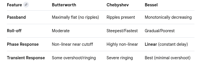
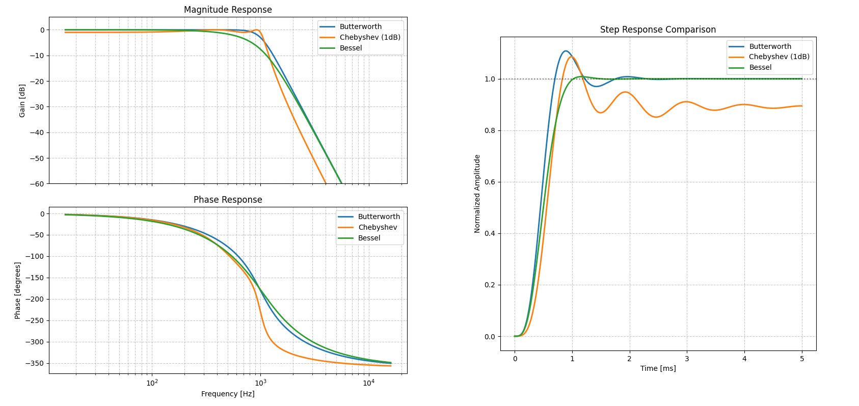
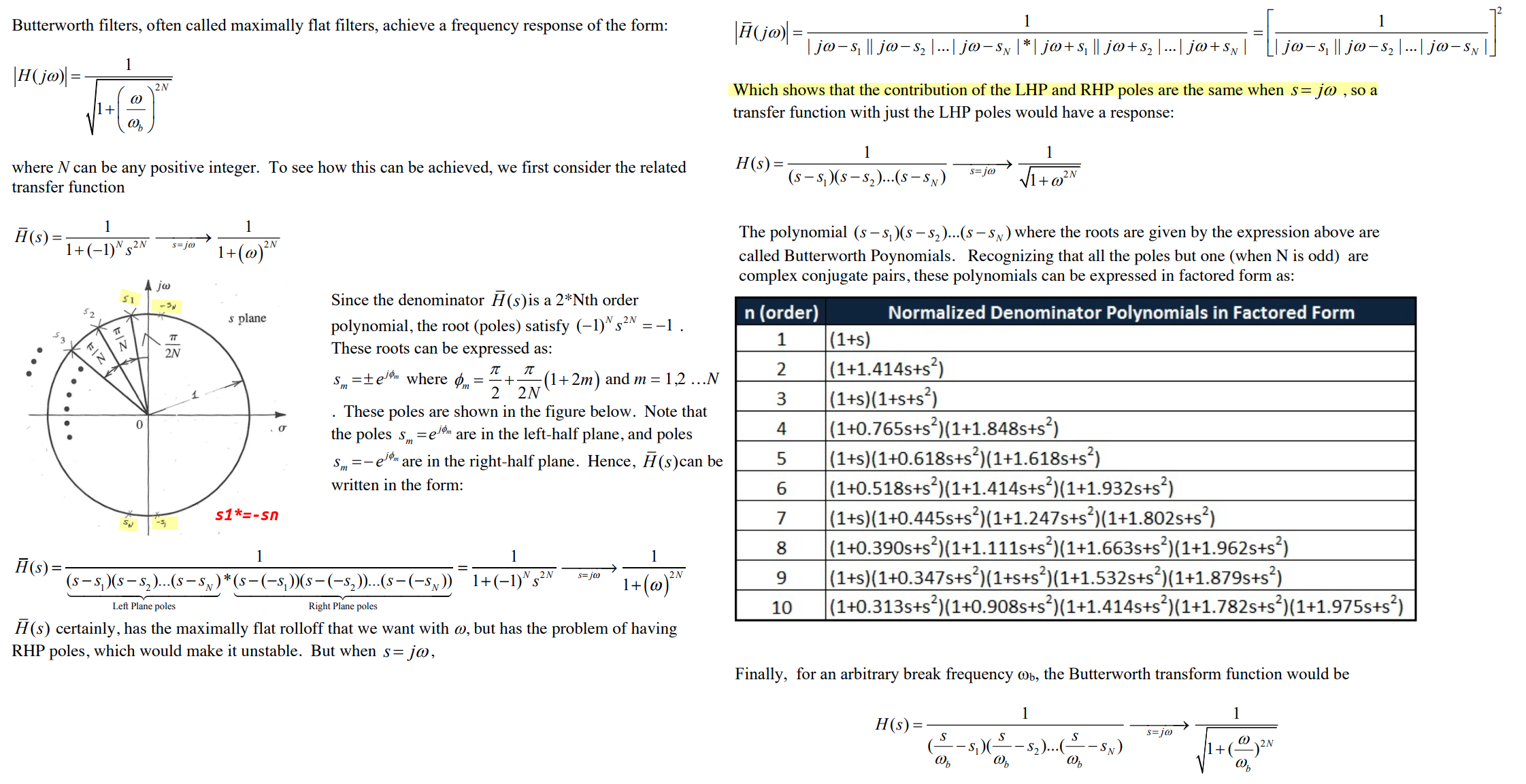
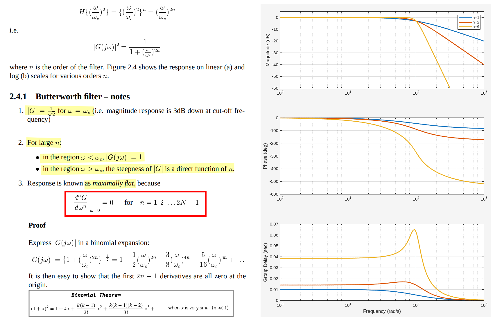
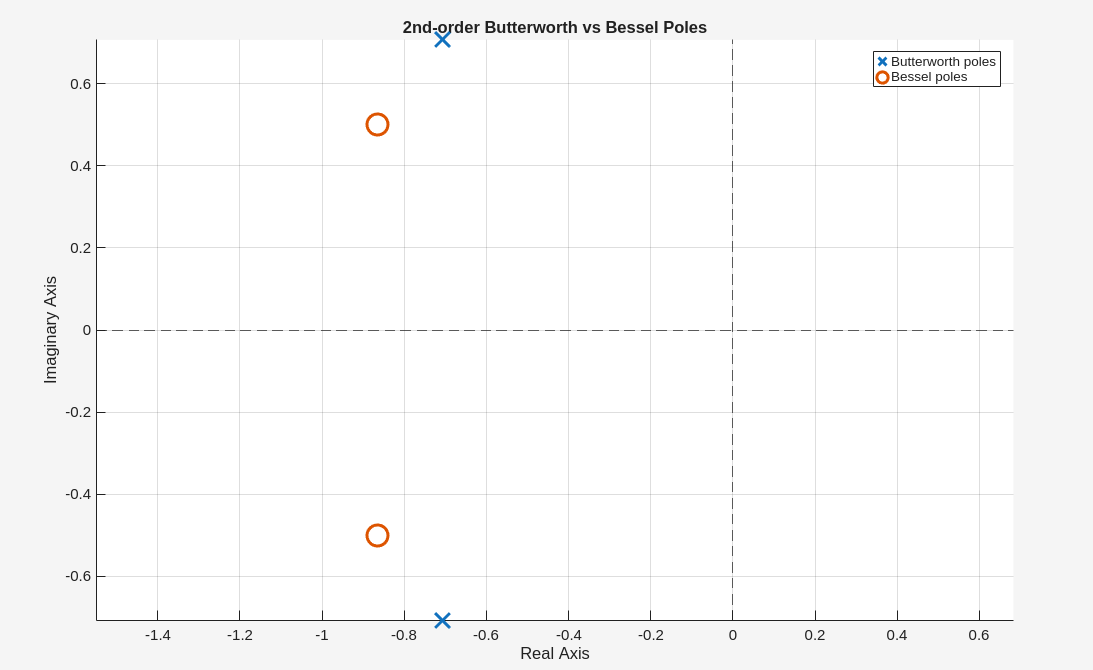
Butterworth Filters
Butterworth Filters [https://people.eecs.ku.edu/~demarest/212/Butterworth%20Filters.pdf]
Stephen Roberts, Signal Processing & Filter Design B3 option: Lecture 2 - Frequency Selective Filters [https://www.robots.ox.ac.uk/~sjrob/Teaching/SP/l2.pdf]
1 | % Parameters |
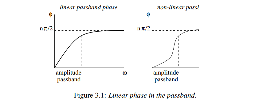
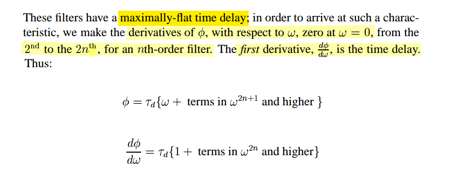
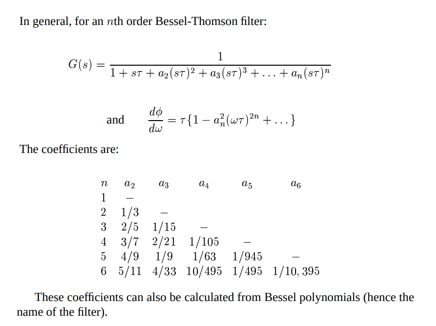
Bessel Filters
Stephen Roberts, Signal Processing & Filter Design B3 option: Lecture 3 - Transient Response and Transforms [https://www.robots.ox.ac.uk/~sjrob/Teaching/SP/l3.pdf]
Bessel filter is often called Bessel–Thomson filter or simply Thomson filter
besself: Bessel analog filter design
[b,a] = besself(n, Wo)
the transfer function coefficients of an \(n\)th-order lowpass analog Bessel filter, where
Wois the angular frequency up to which the filter's group delay is approximately constant. Larger values ofnproduce a group delay that better approximates a constant up toWo.
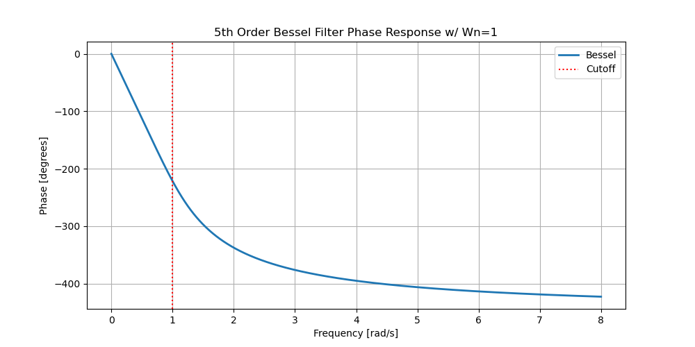
scipy.signal.bessel(N, Wn, btype='low', analog=True, output='ba', norm='phase')
norm='phase'— The filter is normalized such that the phase response reaches its midpoint at angular (e.g. rad/s) frequencyWnThis is the default, and matches MATLAB's implementation.
1 | octave:8> [b,a] = besself(5,1) |
1 | b_bess, a_bess = signal.bessel(5, 1, btype='low', analog=True, norm='phase') |
1 | import numpy as np |
1 | Wn = 1; |
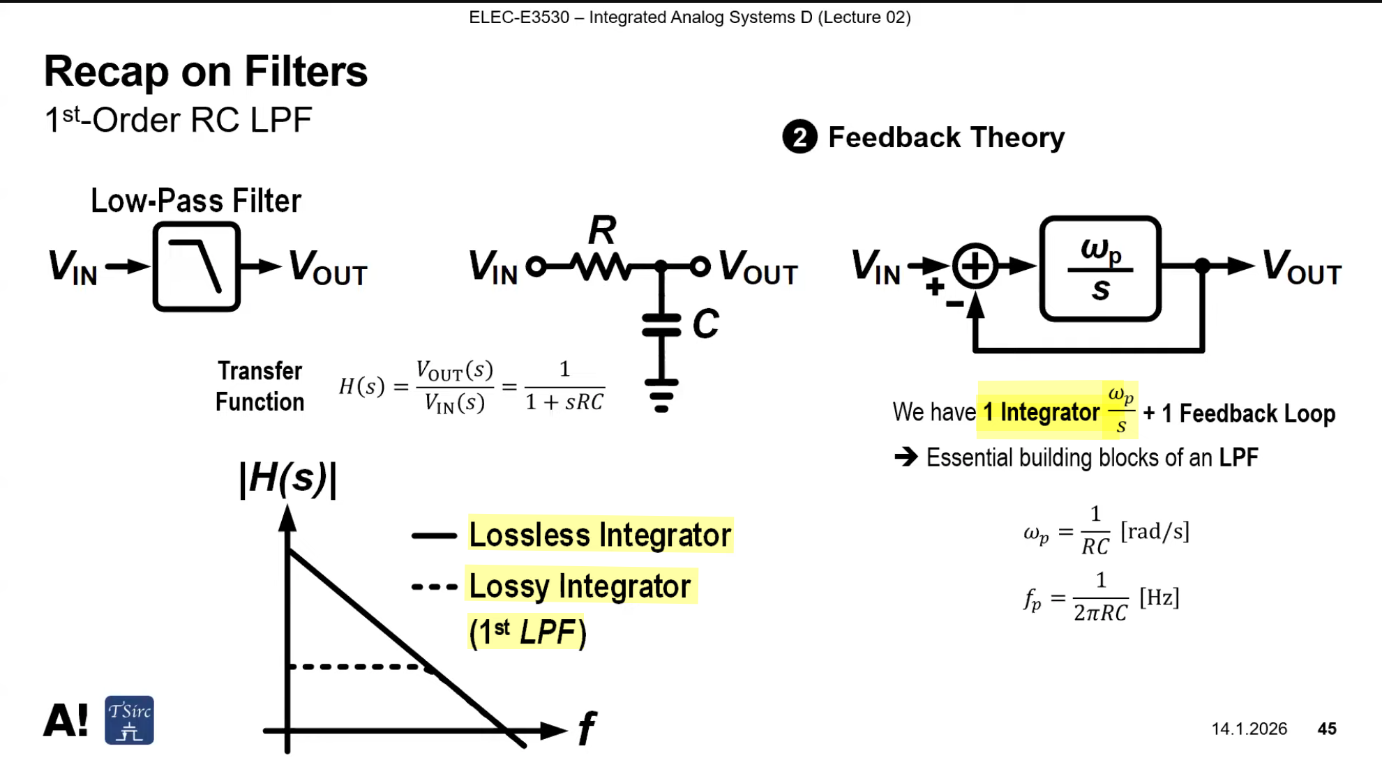
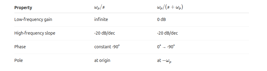
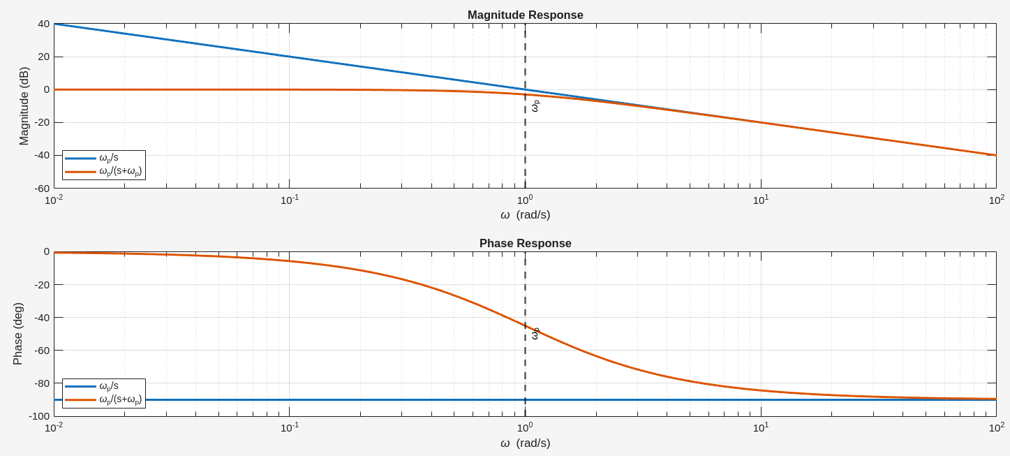
RC LPF
Kwantae Kim, Integrated Analog Systems D - Lecture 02 (Continuous-Time Filters) [https://youtu.be/B7-kr5zV3NA]
—, Integrated Analog Systems D - Lecture 03 (Continuous-Time Filters) [https://youtu.be/6GdDiwaKDZw]
—, Integrated Analog Systems D - Lecture 05 (Continuous-Time Filters) [https://youtu.be/LHhEK1RlC6w]
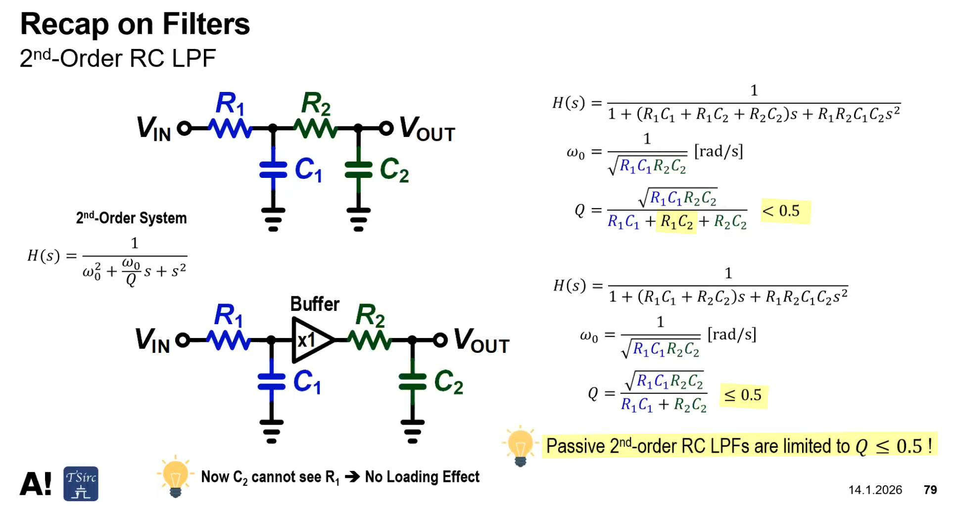
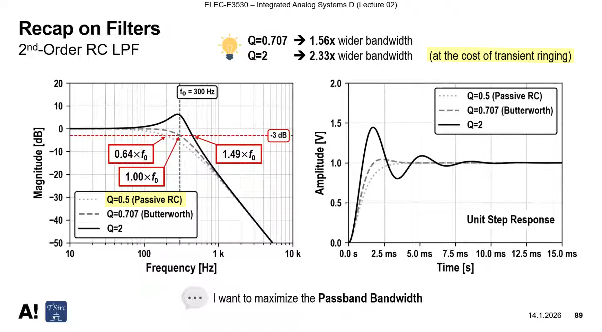
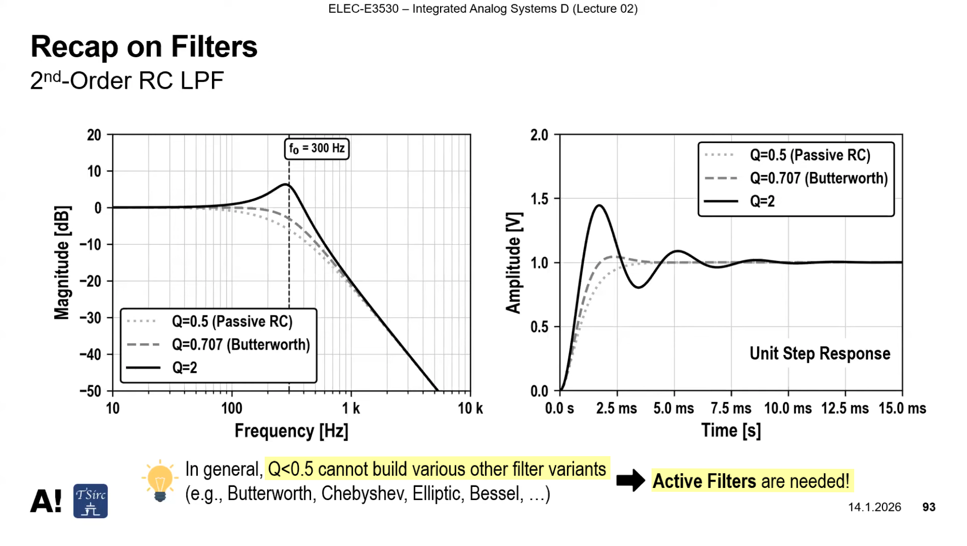
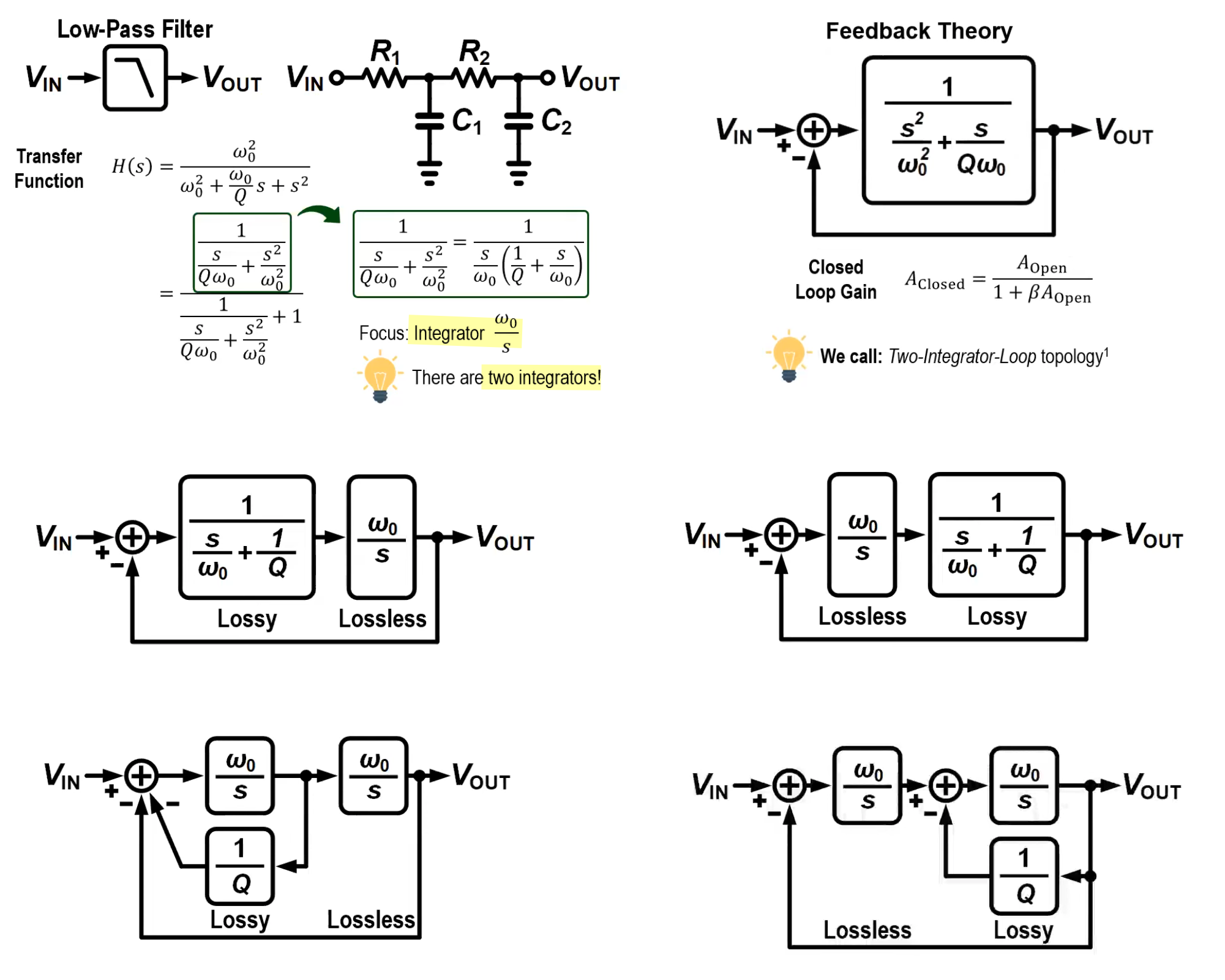
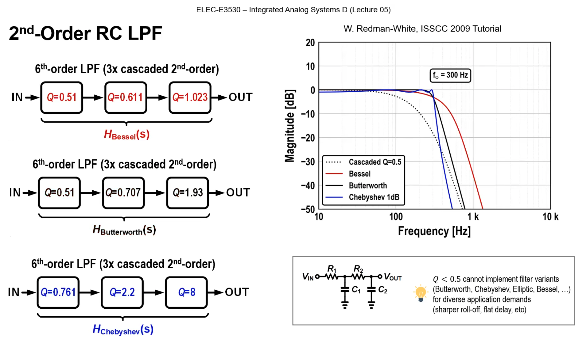
2nd-Order RC LPF
Loading effect & limitation

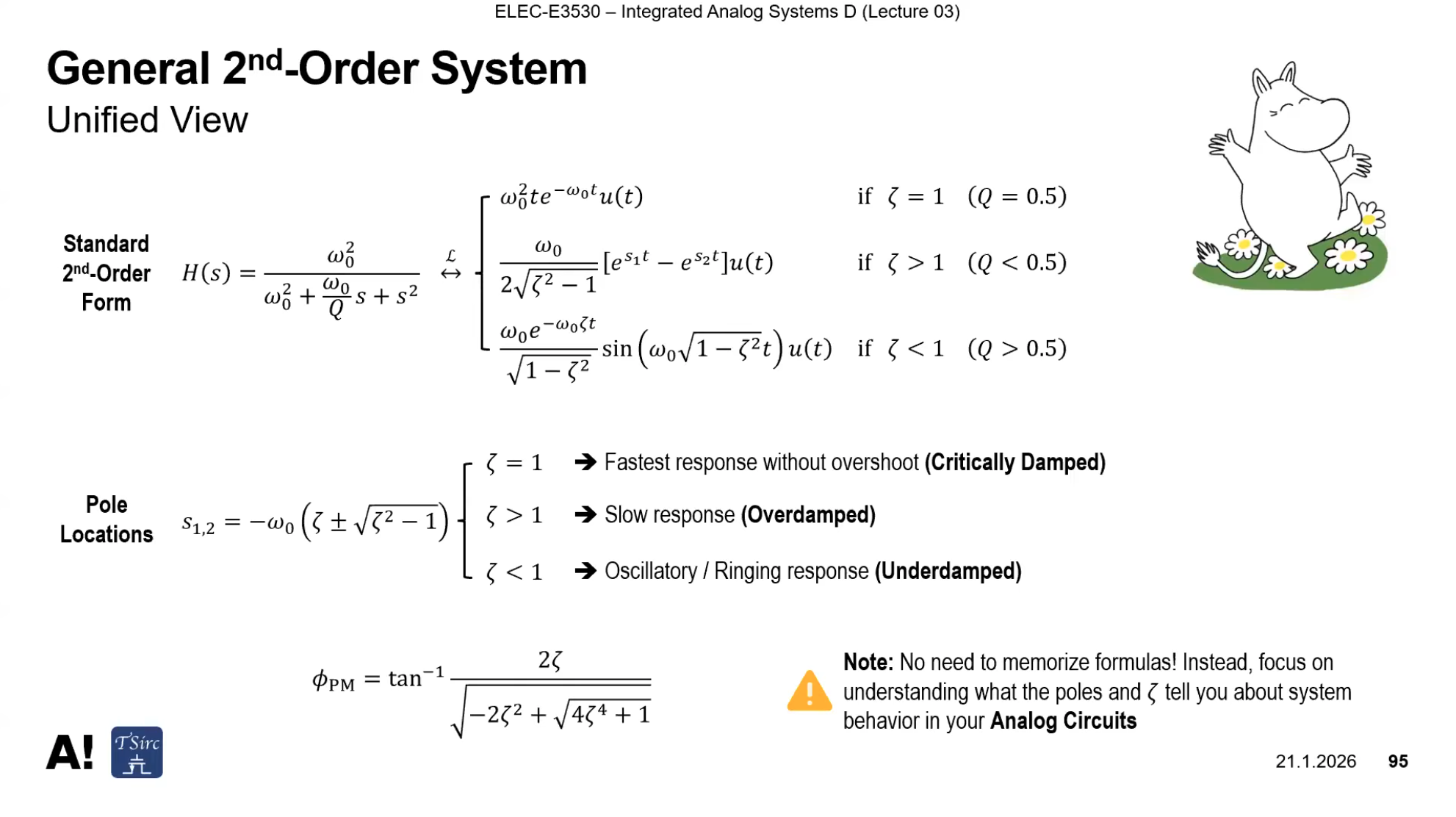
Phase Magin with damping Factor \(\zeta\)
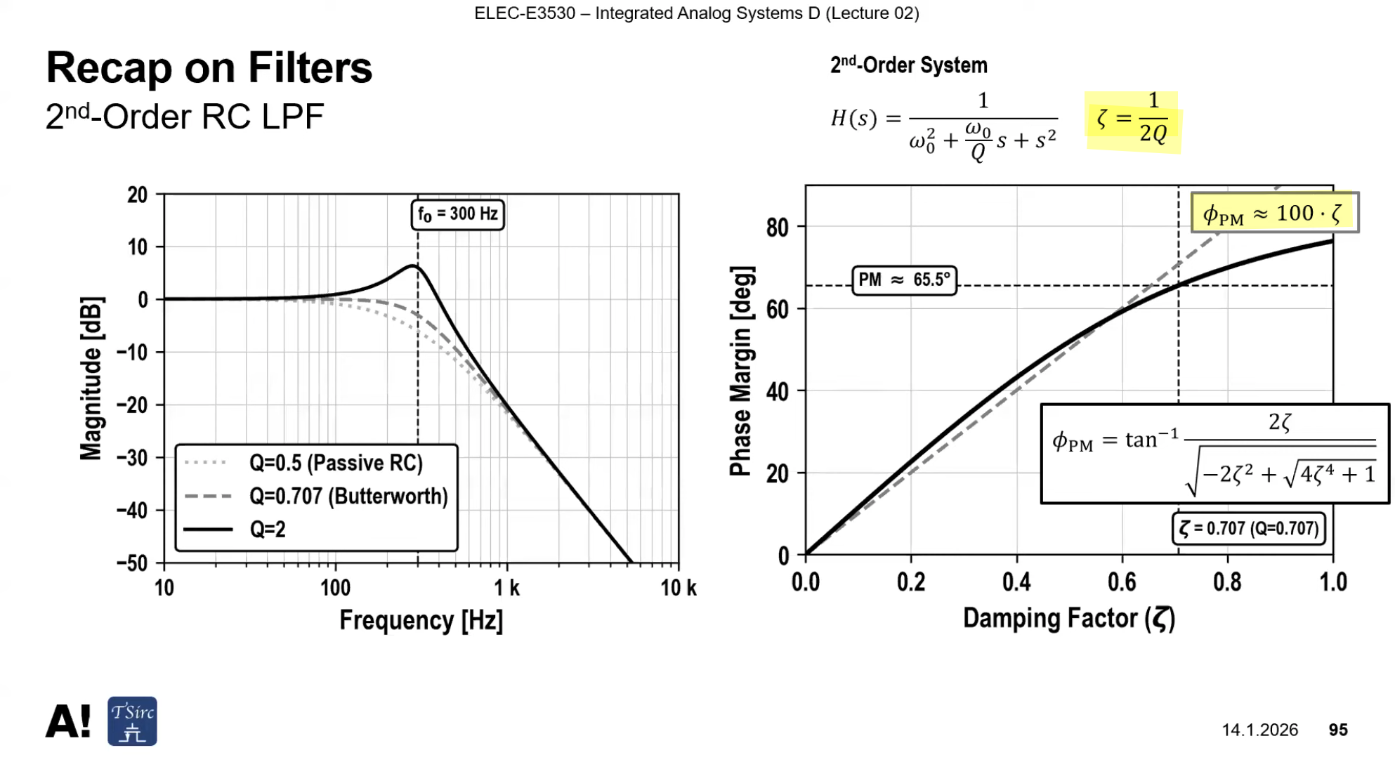 \[
\boxed{\phi_\text{PM}\approx 100\cdot \zeta}
\]
\[
\boxed{\phi_\text{PM}\approx 100\cdot \zeta}
\]
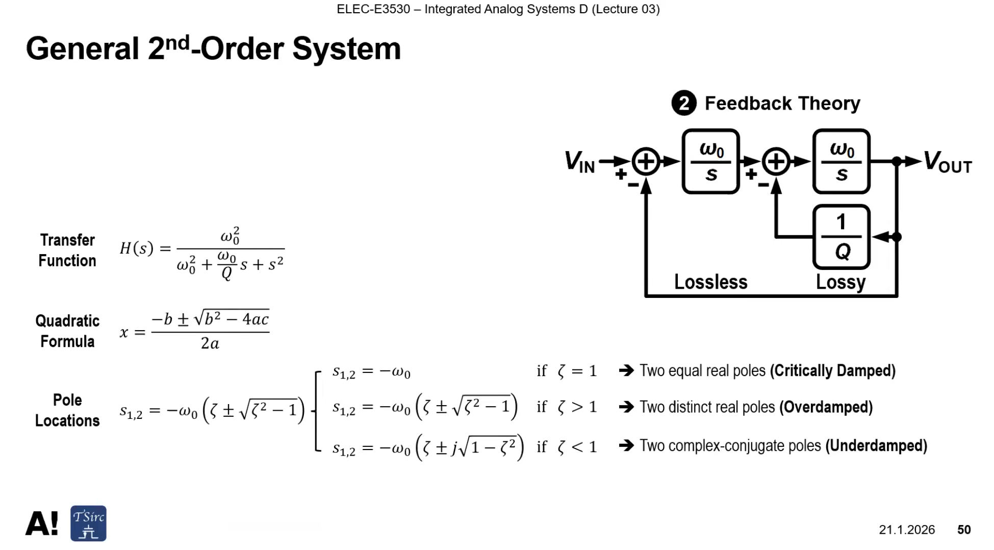
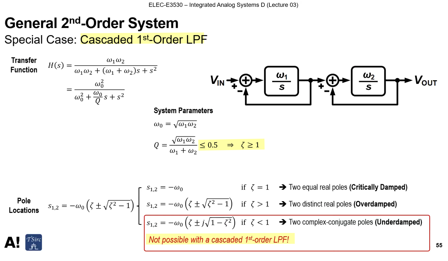
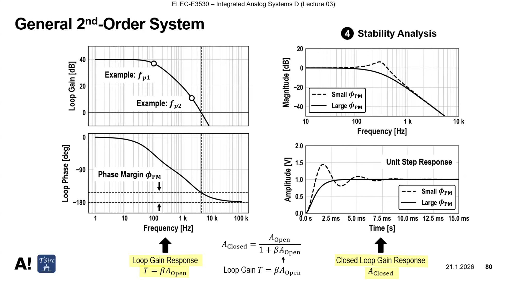
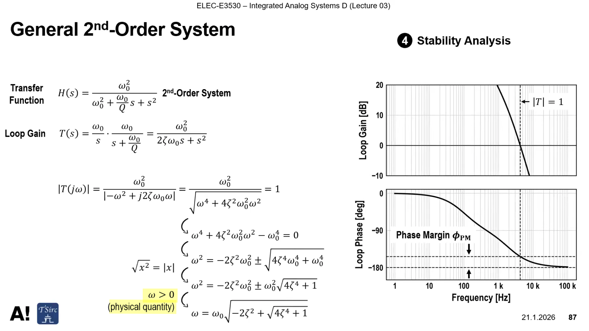
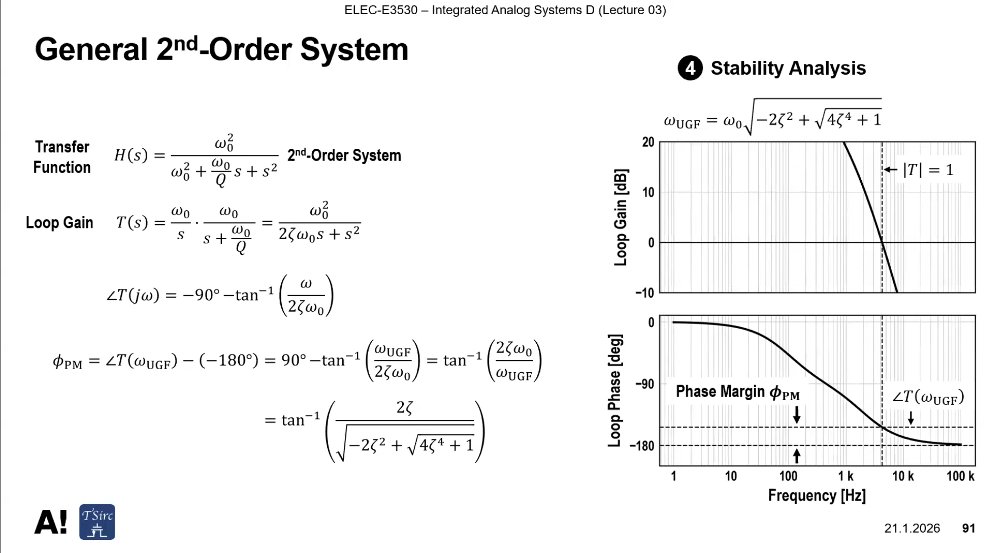
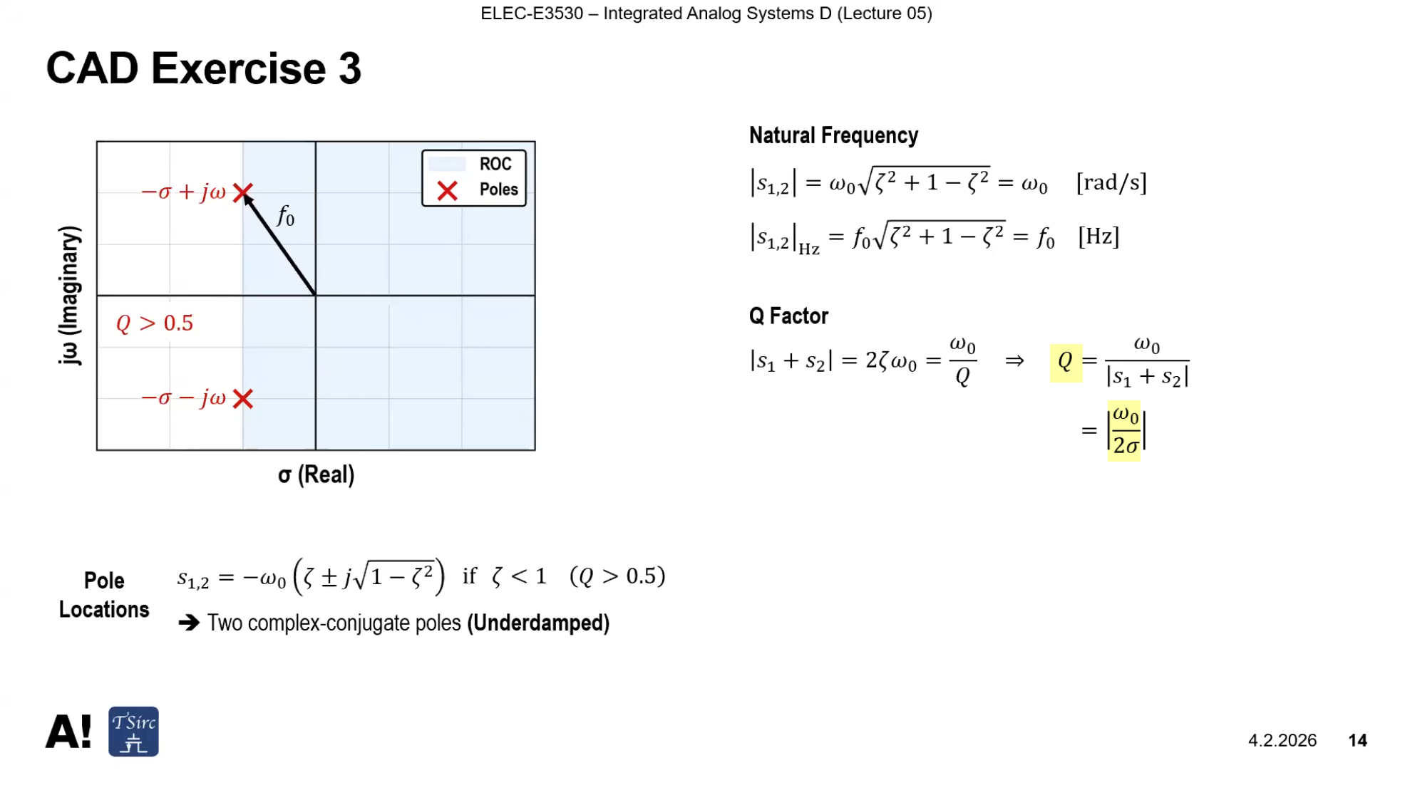
General 2nd-Order RC LPF
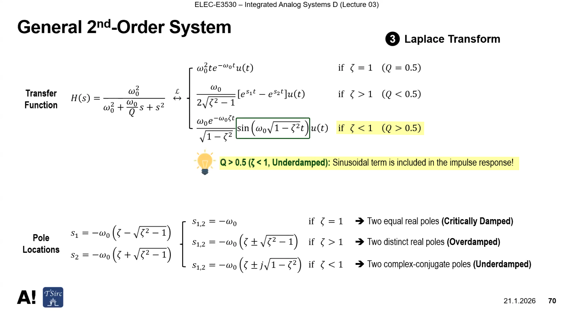
Laplace Transform
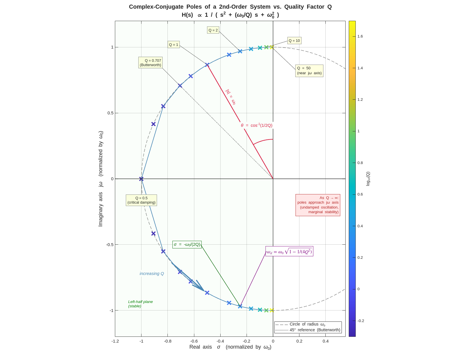
Stability Analysis
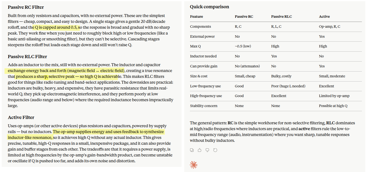
Active Filters
Kwantae Kim, Integrated Analog Systems D - Lecture 05 (Continuous-Time Filters) [https://youtu.be/LHhEK1RlC6w]
TODO 📅
Single-Pole LPF Algorithms
Neil Robertson, Model a Sigma-Delta DAC Plus RC Filter [https://www.dsprelated.com/showarticle/1642.php]
Jason Sachs, Ten Little Algorithms, Part 2: The Single-Pole Low-Pass Filter [https://www.embeddedrelated.com/showarticle/779.php]
—. Return of the Delta-Sigma Modulators, Part 1: Modulation [https://www.dsprelated.com/showarticle/1517/return-of-the-delta-sigma-modulators-part-1-modulation]
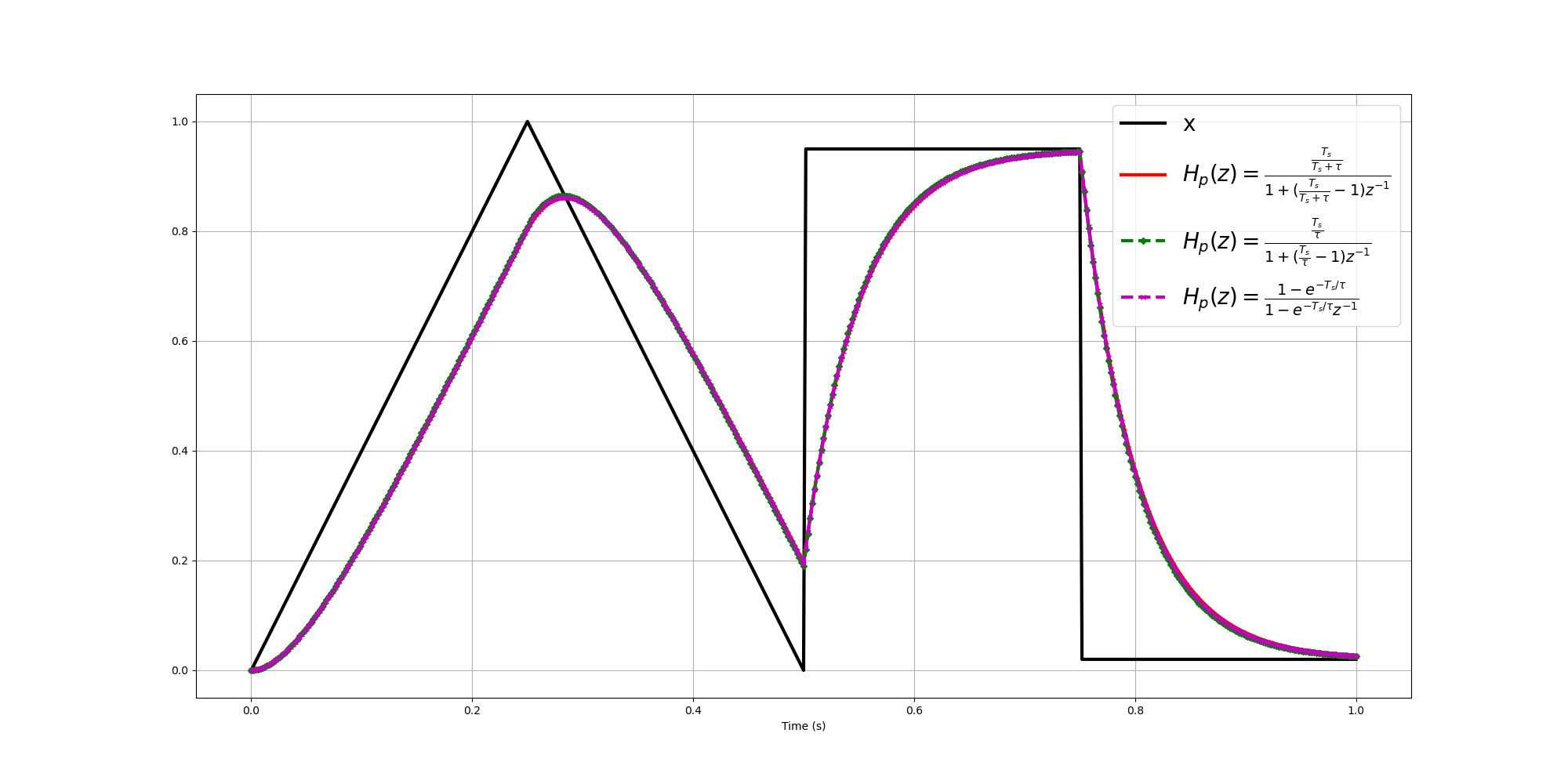
Derivatives Approximation (\(H_p(s)=\frac{1}{s\tau +1}\))
\[\begin{align} H_p(z)&=\frac{\frac{T_s}{T_s+\tau}}{1+(\frac{T_s}{T_s+\tau}-1)z^{-1}}\tag{EQ-0}\\ H_p(z)&=\frac{\frac{T_s}{\tau}}{1+(\frac{T_s}{\tau}-1)z^{-1}}\tag{EQ-1} \end{align}\]
Matched z-Transform (Root Matching) \[ H_p(z)=\frac{1-e^{-T_s/\tau}}{1-e^{-T_s/\tau}z^{-1}}\tag{EQ-2} \] EQ-2 is connected with EQ-1 by \(1 - e^{-\Delta t/\tau} \approx \frac{\Delta t}{\tau}\)
1 | import numpy as np |
1 | x(t) ──┬── R ──┬── y(t) |
Three discretizations of the same continuous prototype, all valid first-order LPFs but with different sample-domain behavior \(\alpha = \frac{T}{T+\tau}\):
| Form | Difference equation | Transfer function | Notes |
|---|---|---|---|
| Backward Euler (above) | \(y_n = (1-\alpha) y_{n-1} + \alpha\, x_n\) | \(\dfrac{\alpha}{1 - (1-\alpha) z^{-1}}\) | Implicit; needs \(x_n\) before computing \(y_n\) |
| Delayed leaky integrator | \(y_n = (1-\alpha) y_{n-1} + \alpha\, x_{n-1}\) | \(\dfrac{\alpha z^{-1}}{1 - (1-\alpha) z^{-1}}\) | One extra sample of delay; same magnitude response |
| Bilinear (Tustin) | \(y_n = (1-\alpha)y_{n-1} + \tfrac{\alpha}{2}(x_n + x_{n-1})\) | \(\dfrac{(\alpha/2)(1 + z^{-1})}{1 - (1-\alpha) z^{-1}}\) | Adds zero at \(z = -1\); better frequency-response match |
| Forward Euler | \(y_n = (1 - T/\tau)y_{n-1} + (T/\tau)\,x_{n-1}\) | \(\dfrac{(T/\tau) z^{-1}}{1 - (1 - T/\tau) z^{-1}}\) | Unstable when \(T > 2\tau\) |
Pole magnitude \(|1-\alpha| < 1\) always — backward Euler is unconditionally stable, unlike forward Euler (\(\alpha = T/\tau\)), which goes unstable when \(T > 2\tau\)
All four collapse to the same continuous-time filter as \(T \to 0\), but they're not interchangeable at finite \(T\) — the delayed leaky integrator in particular adds one sample of group delay that the others don't.
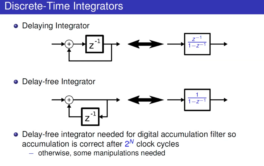
Discrete-Time Integrators
Qasim Chaudhari. Discrete-Time Integrators [https://wirelesspi.com/discrete-time-integrators/]
David Johns (University of Toronto) "Oversampled Data Converters" Course (2019) [https://youtu.be/qIJ2LORYmyA]
Delaying Integrator
Delay-free Integrator
Discrete-Time Differentiator
Qasim Chaudhari. Design of a Discrete-Time Differentiator [https://wirelesspi.com/design-of-a-discrete-time-differentiator/]
TODO 📅
reference
Boris Murmann. EE315A VLSI Signal Conditioning Circuits
Bill Redman-White, ISSCC 2009 Tutorial: T1 : Continuous-Time Filters
B. Nikolic, "Tutorial: Filtering in RF Transceivers," 2014 IEEE International Solid-State Circuits Conference Digest of Technical Papers (ISSCC), San Francisco, CA, USA, 2014
W. Sansen, "Short Course: Power Limits for Amplifiers and Filters," 2012 IEEE International Solid-State Circuits Conference, San Francisco, CA, USA, 2012
Antonio Liscidini, 2018 New Trends in Analog Filters
M. Babaie, "Tutorial: Role of Current-Mode Passive Mixers and N-Path Filters in RF Receivers," 2023 IEEE International Solid-State Circuits Conference (ISSCC), San Francisco, CA, USA, 2023
Stephen Roberts, Signal Processing & Filter Design B3 option [https://www.robots.ox.ac.uk/~sjrob/Teaching/sp_course.html]
Butterworth, Chebyshev & Bessel filters [https://analogcircuitdesign.com/butterworth-and-chebyshev-filters/]
Qasim Chaudhari. FIR vs IIR Filters – A Practical Comparison [https://wirelesspi.com/fir-vs-iir-filters-a-practical-comparison/]
—. Finite Impulse Response (FIR) Filters [https://wirelesspi.com/finite-impulse-response-fir-filters/]
—. Why FIR Filters have Linear Phase [https://wirelesspi.com/why-fir-filters-have-linear-phase/]
—. Moving Average Filter [https://wirelesspi.com/moving-average-filter/]
—. Cascaded Integrator Comb (CIC) Filters – A Staircase of DSP. [https://wirelesspi.com/cascaded-integrator-comb-cic-filters-a-staircase-of-dsp/]
Hideo Okawara's Mixed Signal Lecture Series [https://tomverbeure.github.io/2024/01/06/Hideo-Okawara-Mixed-Signal-Lecture-Series.html]
How to generate complex poles without inductor? [https://a2d2ic.wordpress.com/2020/02/19/basics-on-active-rc-low-pass-filters/]