Noise in Nonlinear Circuits And Systems
A dynamical system can be linear or nonlinear. Independently, it can be deterministic or stochastic. Continuous-time deterministic systems are commonly modeled by ODEs, while continuous-time stochastic systems are commonly modeled by SDEs
| Deterministic | Stochastic | |
|---|---|---|
| Linear | Linear ODE | Linear SDE |
| Nonlinear | Nonlinear ODE | Nonlinear SDE |
The two classifications answer different questions:
- Linear/nonlinear: How does the state enter the evolution equation?
- Deterministic/stochastic: Does the evolution include randomness?
For Demir’s oscillator theory, however, the main path is \[ \boxed{ \text{nonlinear deterministic ODE} \rightarrow \text{add device noise} \rightarrow \text{nonlinear SDE} } \]
instantaneous & average PSD
For white noise \(n(t)\)
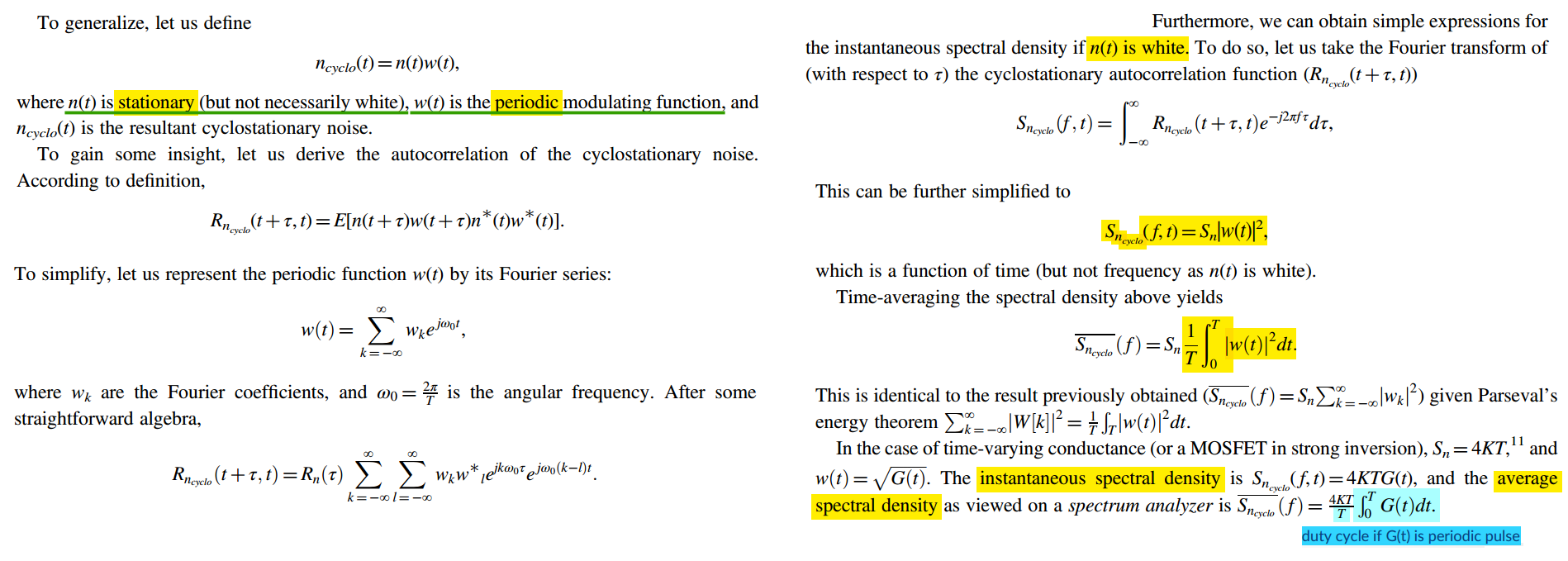
flicker noise Modulation
flicker noise spectrum
Darabi H. Radio Frequency Integrated Circuits and Systems. 2nd ed. Cambridge University Press; 2020.
P. Yelleswarapu, A. Jha, R. Willis, Y. Makris and K. K. O, "Phase Noise Reduction in LC VCO’s Using an Array of Cross-Coupled Nanoscale MOSFETs and Intelligent Post-Fabrication Selection," in IEEE Transactions on Microwave Theory and Techniques, vol. 70, no. 6, pp. 3244-3256, June 2022 [https://sci-hub.ru/10.1109/TMTT.2022.3164949]
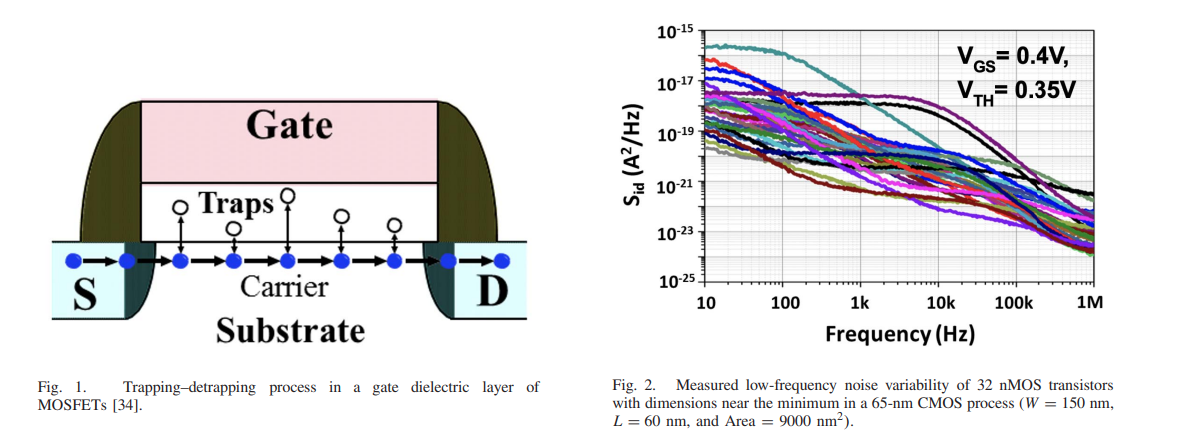
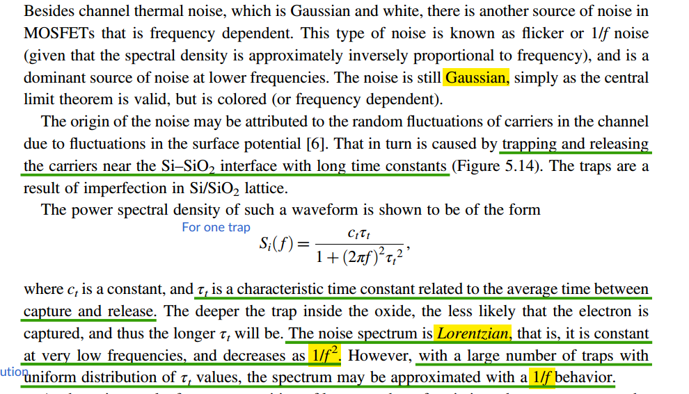
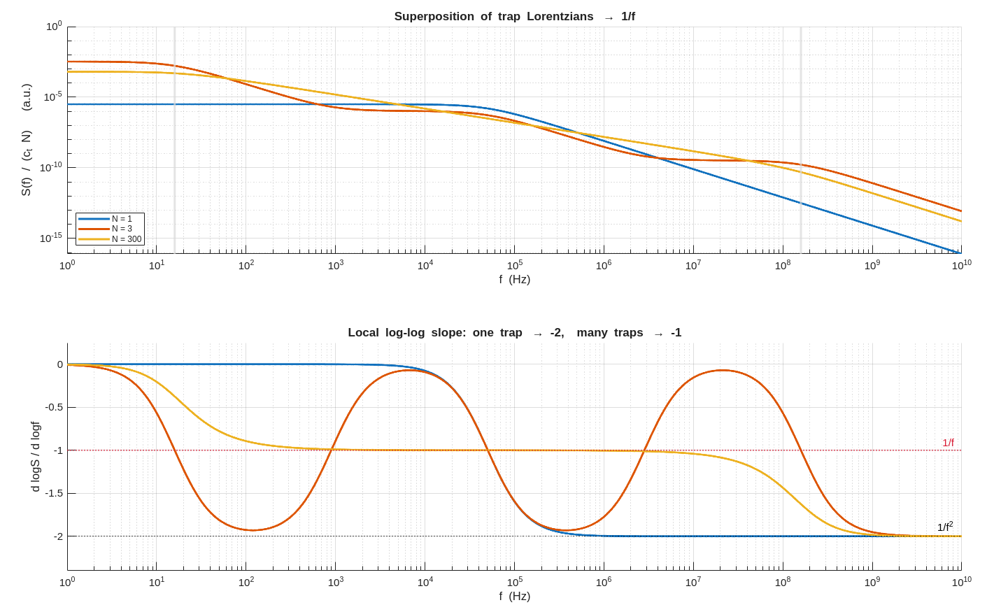
1 | f = logspace(0, 10, 4000); % 1 Hz ... 10 GHz |
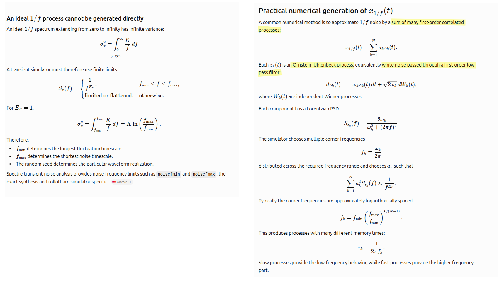
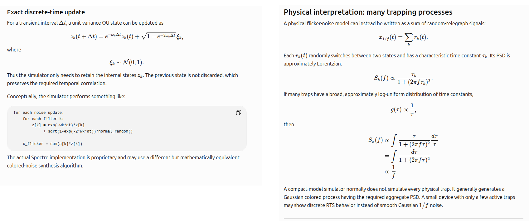
numerical generation of flicker noise
Bibbona, Enrico, Gianna Panfilo and Patrizia Tavella. "The Ornstein–Uhlenbeck process as a model of a low pass filtered white noise." Metrologia 45 (2008): S117 - S126. [https://iris.polito.it/retrieve/e384c42f-3847-d4b2-e053-9f05fe0a1d67/OUasFWN_finale.pdf]
Ornstein–Uhlenbeck process, equivalently white noise passed through a first-order low-pass filter
Flicker Noise Formulations in Verilog-A
G. J. Coram, C. C. McAndrew, K. K. Gullapalli and K. S. Kundert, "Flicker Noise Formulations in Compact Models," in IEEE Transactions on Computer-Aided Design of Integrated Circuits and Systems, vol. 39, no. 10, pp. 2812-2821, Oct. 2020 [https://kenkundert.com/docs/tcad20-flicker-noise.pdf],[https://github.com/KenKundert/flicker-noise]
BSIM4v4.7 MOSFET Model -User's Manual [https://class.ece.iastate.edu/djchen/ee501/BSIM470_Manual.pdf]
C. C. McAndrew et al., "Best Practices for Compact Modeling in Verilog-A," in IEEE Journal of the Electron Devices Society, vol. 3, no. 5, pp. 383-396, Sept. 2015 [https://ieeexplore.ieee.org/stamp/stamp.jsp?arnumber=7154394]
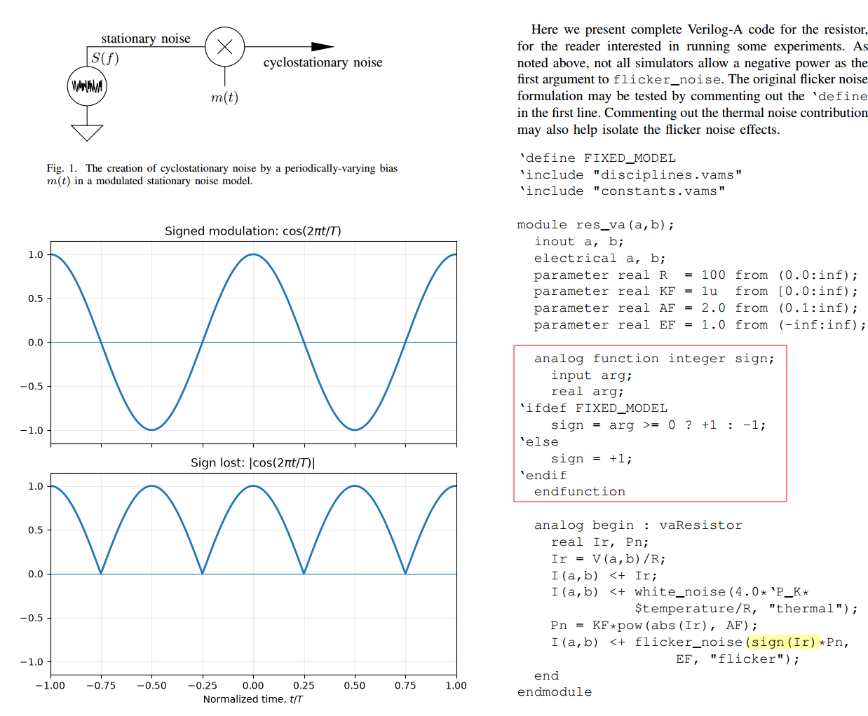
When sign(Ir) = -1, the argument becomes \[
q(t)=\operatorname{sign}(I_r)P_n=-P_n.
\] A simulator that correctly supports Kundert’s formulation does
not interpret this as a physically negative PSD, nor
does it calculate the ordinary complex square root \(\sqrt{-P_n}\). Instead, the sign selects
the sign of the deterministic noise-modulation amplitude: \[
\boxed{
m(t)=\operatorname{sign}\!\big(q(t)\big)\sqrt{|q(t)|}
}
\] Therefore, when \(q=-P_n\),
\[
m(t)=-\sqrt{P_n}.
\] This is equivalent to
1 | I(a,b) <+ sign(Ir)*flicker_noise(Pn, EF, "flicker"); |
provided the simulator supports a noise function inside an expression
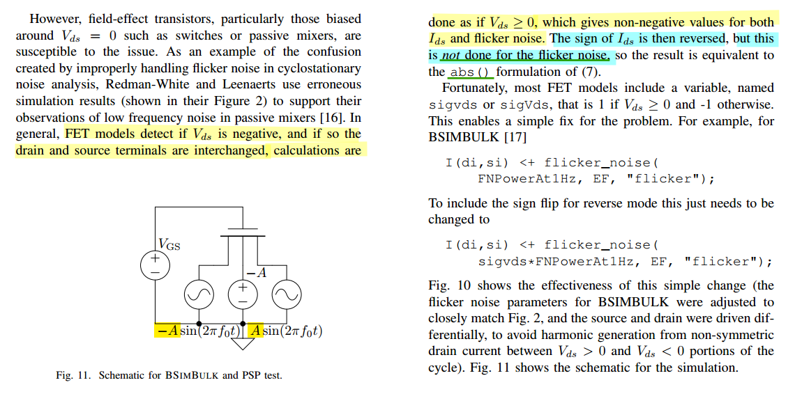
1 | // BSIM flicker noise simulations |
1 | // Resistor flicker noise simulations |
Marek Mierzwinski, Verilog-A Standardization for Compact Modeling [https://www.mos-ak.org/washington_dc/papers/Mierzwinski_MOS-AK_2011.pdf]
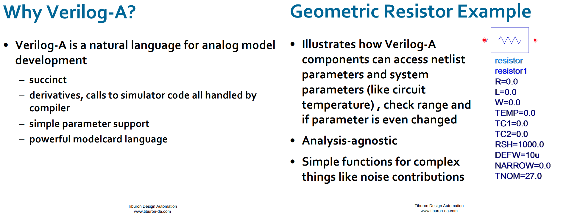
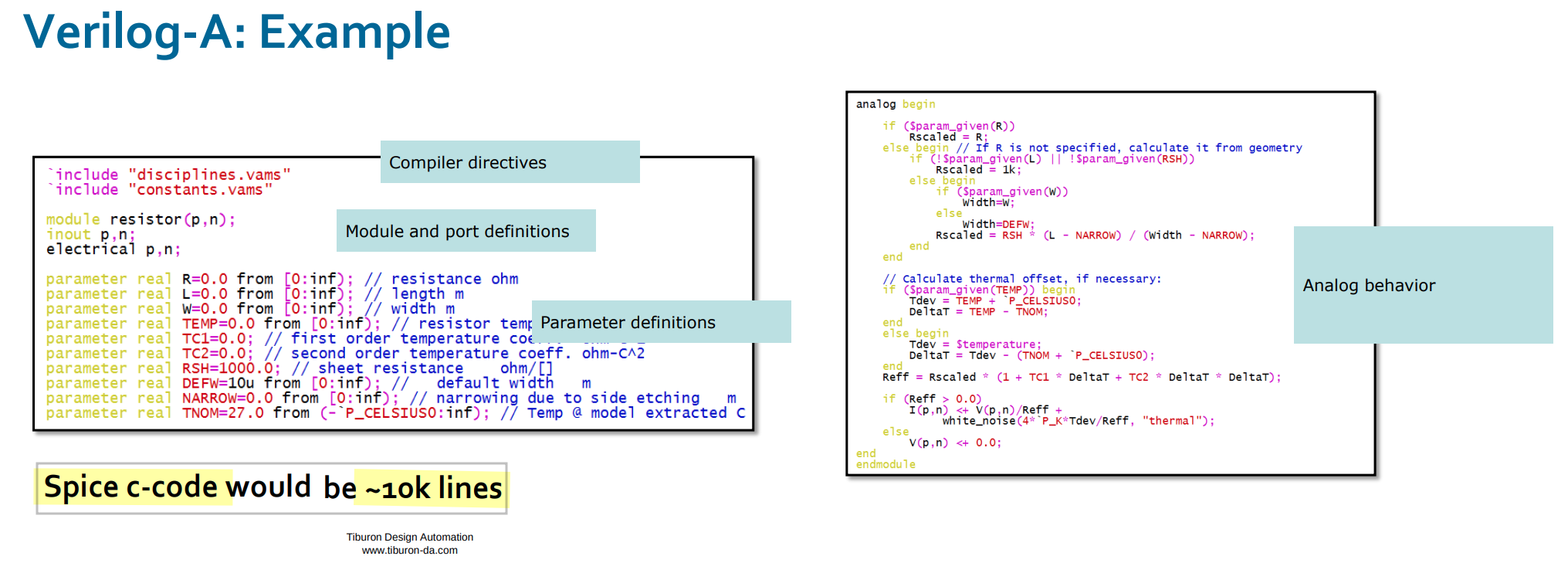
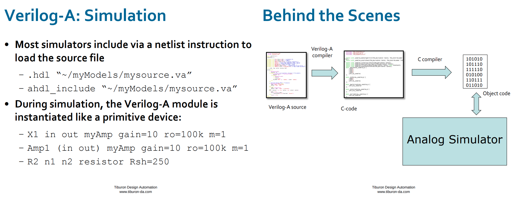
Current BSIM models use compact-model equations standardized through reference Verilog-A code, but commercial simulators often execute an optimized built-in implementation rather than the Verilog-A source directly
flicker noise in circuit-noise analysis
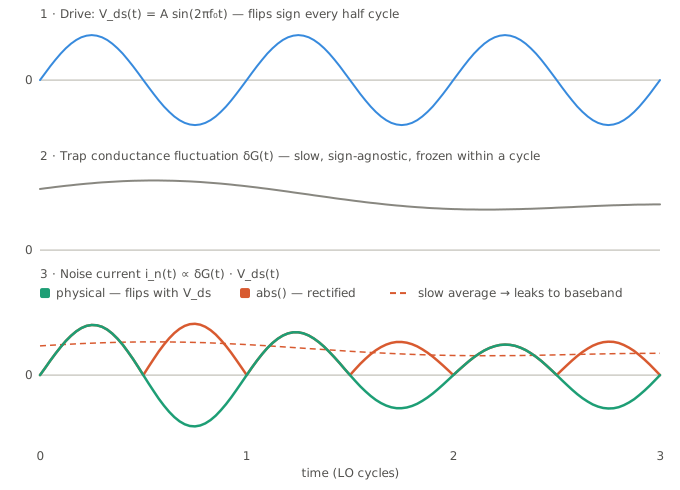
its power spectral density is approximately \[ S_{i,1/f}(f)=\frac{K}{|f|}. \] A large amount of its power lies at low frequencies. Therefore, compared with a GHz oscillation period \(T_0\), the flicker-noise value changes very little during one cycle.
For a flicker-noise component at frequency \(f_m\), \[ f_m T_0\ll 1 \] implies \[ i_{1/f}(t+T_0)\approx i_{1/f}(t). \] Thus, if the noise current is positive at \(t_0\), it will probably remain positive throughout the following oscillator cycle: \[ i_{1/f}(t_0+\tau)\approx i_{1/f}(t_0), \qquad 0\leq \tau<T_0. \] In circuit-noise analysis, the underlying flicker-noise source is commonly treated as approximately wide-sense stationary: \[ R_x(t_1,t_2)=R_x(t_1-t_2). \] This is reasonable when the device bias is constant and the measurement interval is finite.
The phase perturbations may cancel or leave a nonzero residual: \[ \Delta\phi_{\text{cycle}} \propto \int_{0}^{T_0} \Gamma(\omega_0 t)\, i_{1/f,\mathrm{cyclo}}(t)\,dt. \] Since the low-frequency noise is almost constant over \(T_0\), \[ \Delta\phi_{\text{cycle}} \approx x_{1/f}(t_0) \int_{0}^{T_0} \Gamma(\omega_0 t)a(t)\,dt \] Therefore, flicker-noise upconversion depends on whether the phase-delay and phase-advance contributions cancel over one period. A nonzero weighted average produces low-frequency fluctuations in oscillator frequency, which commonly appear as the \(1/f^3\) phase-noise region.
Define
\[ \Gamma_{\mathrm{eff,DC}}\equiv \frac{1}{T_0}\int_0^{T_0}\Gamma(\omega_0t)a(t)\,dt \]
Then \[ \Delta\phi_{\text{cycle}} \approx \frac{x_{1/f}(t_0)}{q_{\max}} \Gamma_{\mathrm{eff,DC}}T_0. \] If \(x_{1/f}\) is already normalized by \(q_{\max}\), the \(1/q_{\max}\) factor can be omitted.
Therefore, \[ \boxed{\Gamma_{\mathrm{eff,DC}}=0 \quad\Longrightarrow\quad \Delta\phi_{\text{cycle}}\approx 0} \] for quasistatic flicker noise. Physically, the phase-delay contribution on one edge exactly cancels the phase-advance contribution on the other edge.nce, \[ \boxed{ \Gamma_{\mathrm{eff,DC}}=0 \Rightarrow \text{no first-order direct }1/f\text{-to-}1/f^3 \text{ phase-noise upconversion from that source.} } \]
Ordinary Differential Equations (ODEs)
Steve Brunton, ME 564 - Mechanical Engineering Analysis [http://faculty.washington.edu/sbrunton/me564/] [videos]
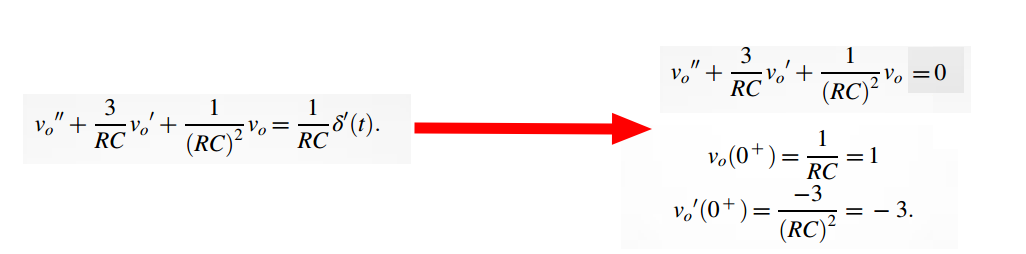
Dirac delta function in ODEs
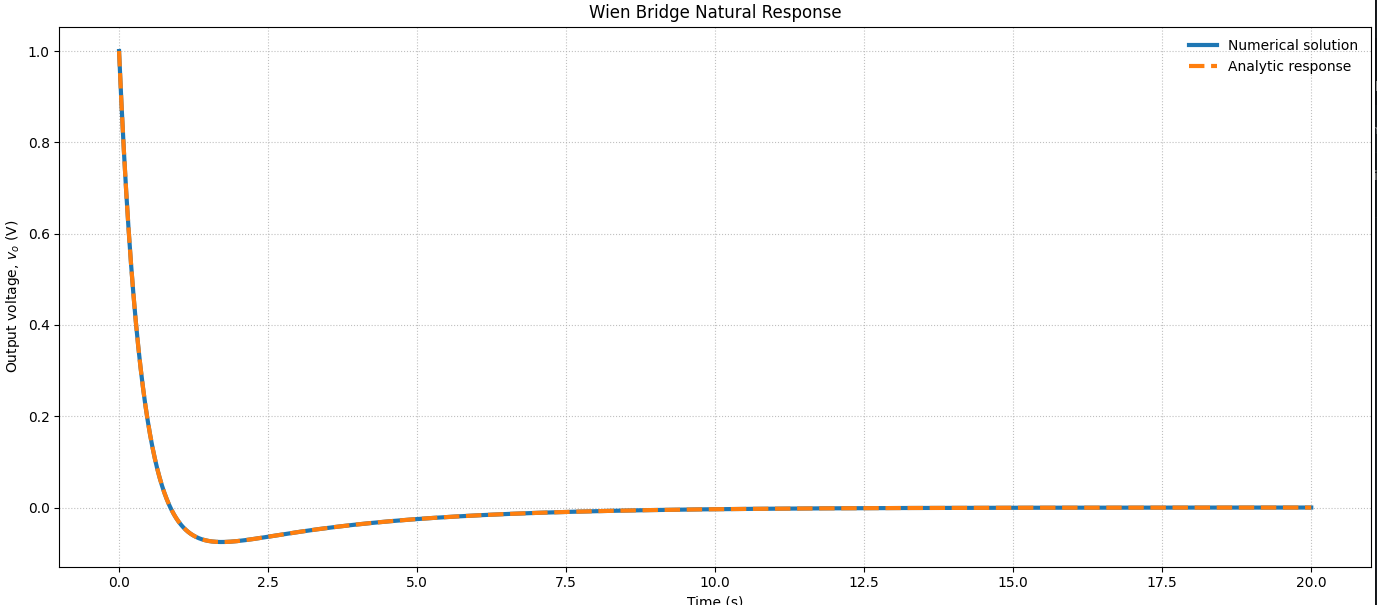
Integrate across the impulse to find the jump \[ \underbrace{\text{zero state} + \delta(t)\text{ input}}_{t=0^-} \quad\Longrightarrow\quad \underbrace{\text{zero input} + \text{new ICs at }t=0^+}_{t>0} \]
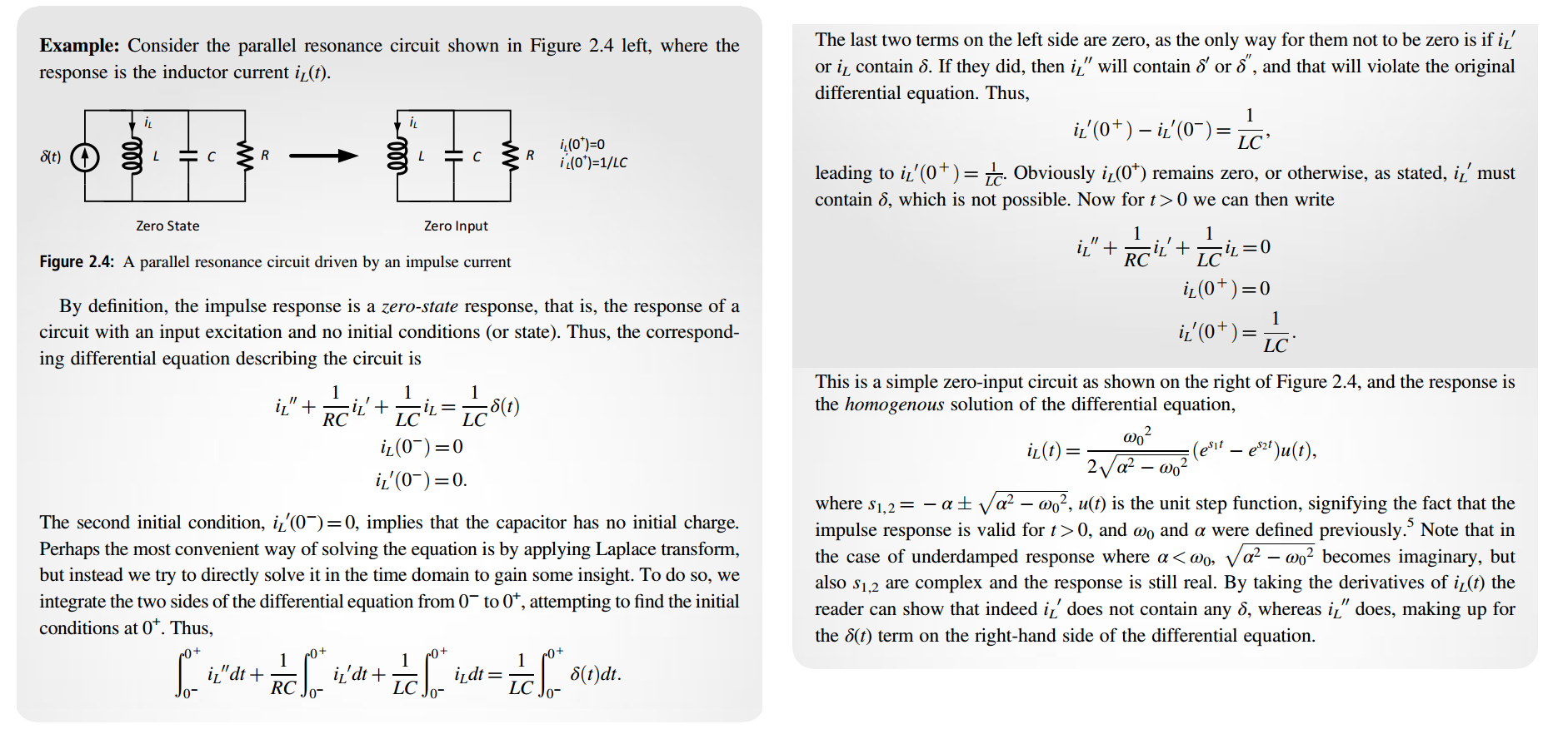
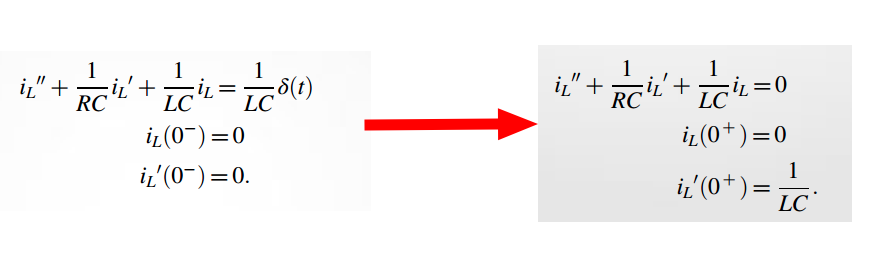
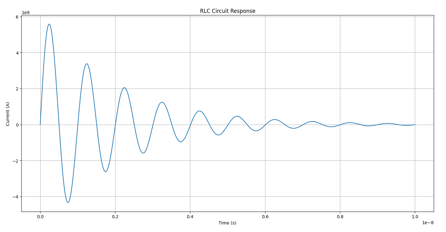
1 | import numpy as np |
Doublet function in ODEs
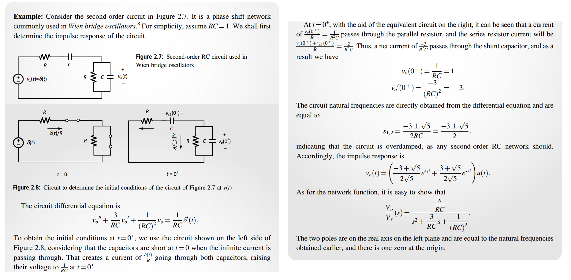
1 | import numpy as np |
Stochastic Differential Equations (SDE)
TODO 📅
Fourier Analysis & Partial Differential Equations (PDEs)
\[ \text{Fourier analysis} \longrightarrow \text{method for solving PDEs}, \]
TODO 📅
Differential Equations in Matlab & Python
scipy.integrate.solve_ivp
Solve an initial value problem for a system of ODEs
rtol and atol are the error tolerances for
scipy.integrate.solve_ivp.
rtol is relative tolerance: allowed error scales with
the size of the solution.
atol is absolute tolerance: allowed error floor when the
solution is near zero.
SciPy roughly controls local error using:
1 | error < atol + rtol * abs(y) |
DifferentialEquations.jl
ODE forms
ODE is usually defined in one of two forms: out-of-place or in-place
1 | # out-of-place |
x = current state
p = parameters
t = current time
returned value = dx/dt
1 | # in-place |
Scalar ODE \[ \frac{dx}{dt} = -2x \]
1 | function f(x, p, t) |
System of ODEs
\[\begin{align} \dot{x} &= y, \\ \dot{y} &= -x - 0.2y. \end{align}\]
1 | function oscillator!(du, u, p, t) |
\[ u = \begin{bmatrix} x \\ y \end{bmatrix}, \quad du = \begin{bmatrix} \dot{x} \\ \dot{y} \end{bmatrix}. \]
ODE with parameters
1 | function f!(du, u, p, t) |
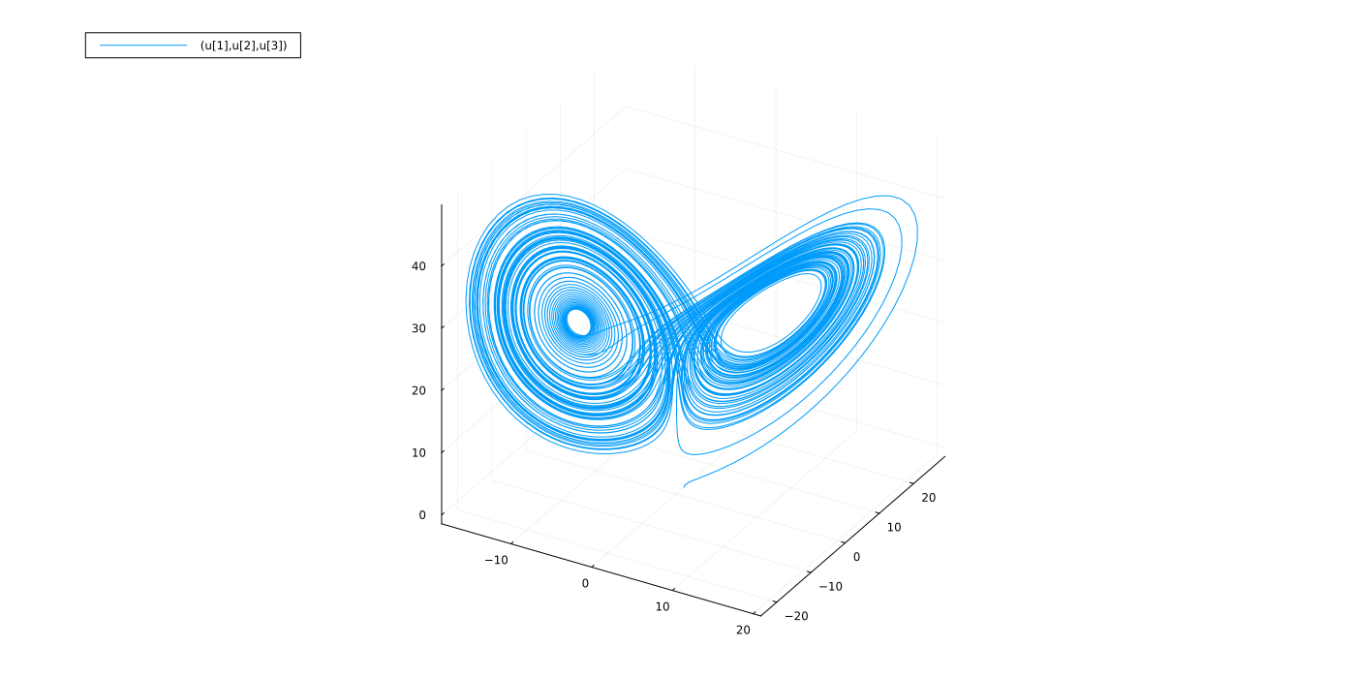
The Lorenz Equation — employ above features
\[\begin{align} \frac{dx}{dt} &= \sigma (y - x) \\ \frac{dy}{dt} &= x (\rho - z) -y \\ \frac{dz}{dt} &= xy - \beta z \end{align}\]
1 | function lorenz!(du,u,p,t) |
Event Handling & Callback Functions
In DifferentialEquations.jl, a callback
allows the ODE solver to detect an event and execute some action when
that event occurs. This is useful for hybrid systems, switching
circuits, threshold detection, impacts, resets, stopping conditions,
etc. \[
\boxed{\text{condition} \longrightarrow \text{event} \longrightarrow
\text{affect!}}
\]
| Callback | Condition | Typical use |
|---|---|---|
ContinuousCallback |
(g(u,t)=0) | zero crossings, thresholds, impacts |
DiscreteCallback |
Boolean | mode switching, logical conditions |
1 | function f!(du, u, p, t) |
integrator is the currently running solver
object. DifferentialEquations.jl automatically
passes it into callback functions.
1 | integrator.u # current state |
ContinuousCallback
Use ContinuousCallback when the event is defined by a
continuous zero crossing \(g(u,t)=0\)
graph LR
A[ODE solver] --> B[integrate normally]
B --> C{condition = 0 ?}
C -- yes --> D["affect!()"]
D --> E[continue integration]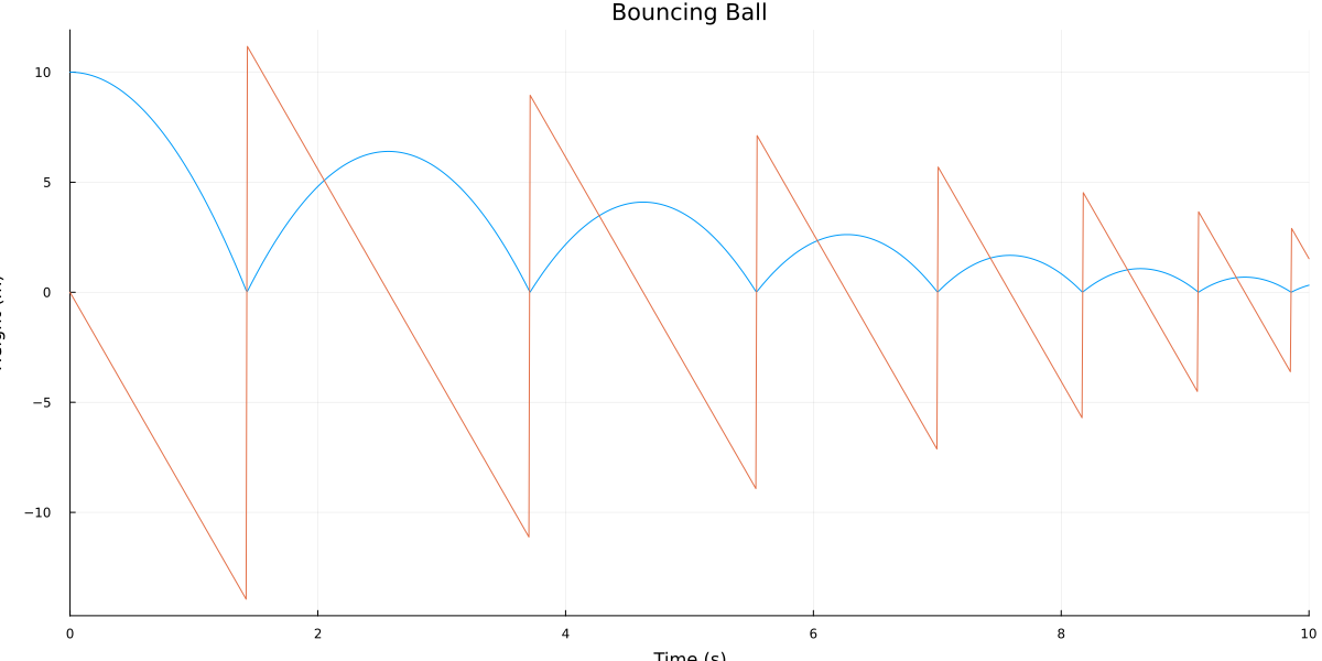 \[
\begin{cases}
\dot{x} = v \\
\dot{v} = -g
\end{cases}
\]
\[
\begin{cases}
\dot{x} = v \\
\dot{v} = -g
\end{cases}
\]
1 | using DifferentialEquations |
DiscreteCallback
The condition returns a Boolean
1 | condition(u, t, integrator) = true/false |
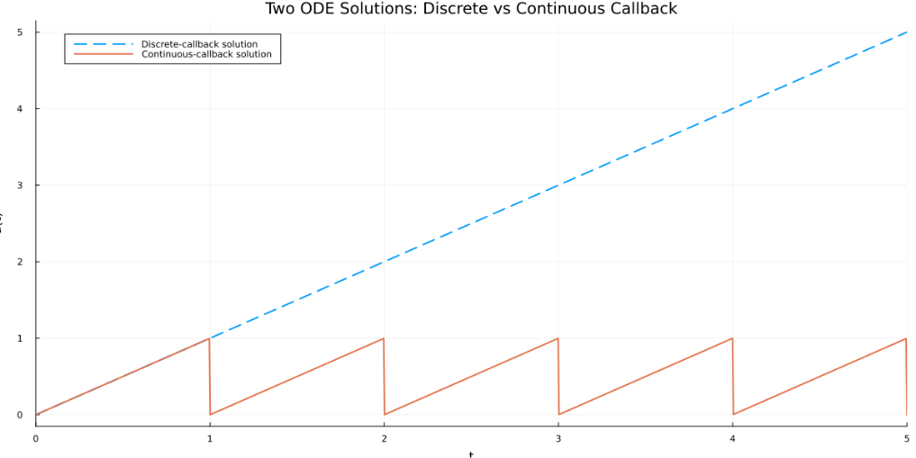
DiscreteCallback checks its Boolean condition at
the end of accepted integration steps. It does not use root
finding to locate the exact point where \(u=1\)
1 | using DifferentialEquations |
DiscreteCallback checks only after each accepted solver
step. Because du/dt = 1 is exactly linear,
Tsit5() takes a large step from approximately
t=0.58 directly to t=5. It therefore does not
check near u=1.
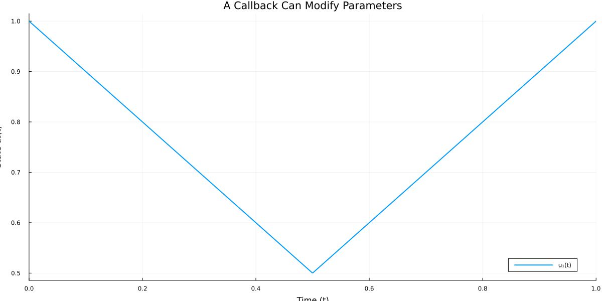
A callback can modify parameters
Callbacks provide the mechanism that connects the continuous ODE dynamics to this discrete switching behavior
So mathematically two components: \[ \dot{\mathbf{x}} = f(\mathbf{x}, p, t) \] for the \(\textbf{continuous-time dynamics}\), and \[ g(\mathbf{x}, t) = 0 \implies (\mathbf{x}, p) \to R(\mathbf{x}, p) \] for the \(\textbf{event/reset dynamics}\). \(R(x,p)\) means a reset map or event update rule
\[ \dot{x} = \begin{cases} -x, & x > 0.5 \\ -2x, & x < 0.5. \end{cases} \]
1 | using DifferentialEquations |
reference
A. Demir, A. Mehrotra and J. Roychowdhury, "Phase noise in oscillators: a unifying theory and numerical methods for characterization," in IEEE Transactions on Circuits and Systems I: Fundamental Theory and Applications, vol. 47, no. 5, pp. 655-674, May 2000 [https://sci-hub.jp/10.1109/81.847872]
—, "A Reliable and Efficient Procedure for Oscillator PPV Computation, With Phase Noise Macromodeling Applications," IEEE TCAD, 2003.
— and A. Sangiovanni-Vincentelli, Analysis and Simulation of Noise in Nonlinear Electronic Circuits and Systems, vol. 425. Boston, MA, USA: Kluwer Academic Publishers, 1998
A. Mehrotra and A. Sangiovanni-Vincentelli, Noise Analysis of Radio Frequency Circuits, 1st ed. New York, NY, USA: Springer, 2004
Mathematical Preliminaries
Strogatz, S.H. (2015). Nonlinear Dynamics and Chaos: With Applications to Physics, Biology, Chemistry, and Engineering (2nd ed.). CRC Press [https://www.biodyn.ro/course/literatura/Nonlinear_Dynamics_and_Chaos_2018_Steven_H._Strogatz.pdf]
Higham, Desmond. (2001). An Algorithmic Introduction to Numerical Simulation of Stochastic Differential Equations. SIAM Review. 43. 525-546. 10.1137/S0036144500378302. [https://www.cmor-faculty.rice.edu/~cox/stoch/dhigham.pdf]
Jiří Lebl. Notes on Diffy Qs: Differential Equations for Engineers [link]
Matt Charnley. Differential Equations: An Introduction for Engineers [link]
Åström, K.J. & Murray, Richard. (2021). Feedback Systems: An Introduction for Scientists and Engineers Second Edition [https://www.cds.caltech.edu/~murray/books/AM08/pdf/fbs-public_24Jul2020.pdf]