Fixed-Point Signal Processing
why fixed-point arithmetic?
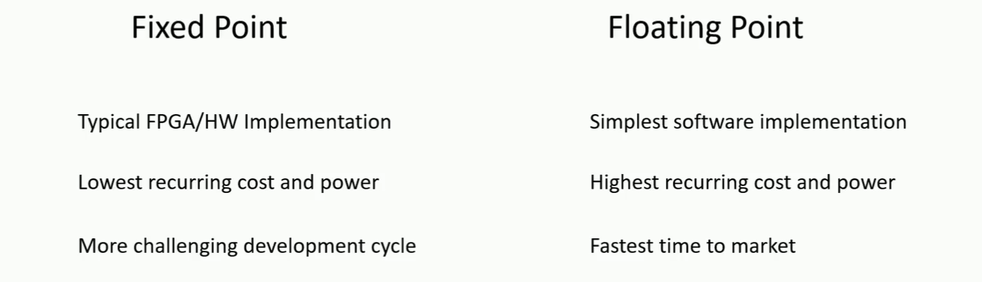
Because the dynamic range of the incoming physical signal is tightly controlled by an Analog Front End (AFE) using Automatic Gain Control (AGC), a massive floating-point dynamic range isn't necessary
Number Systems
Harris, David Money, and Sarah L. Harris. Digital Design and Computer Architecture. 2nd ed. Morgan Kaufmann, 2013. [pdf]
integers
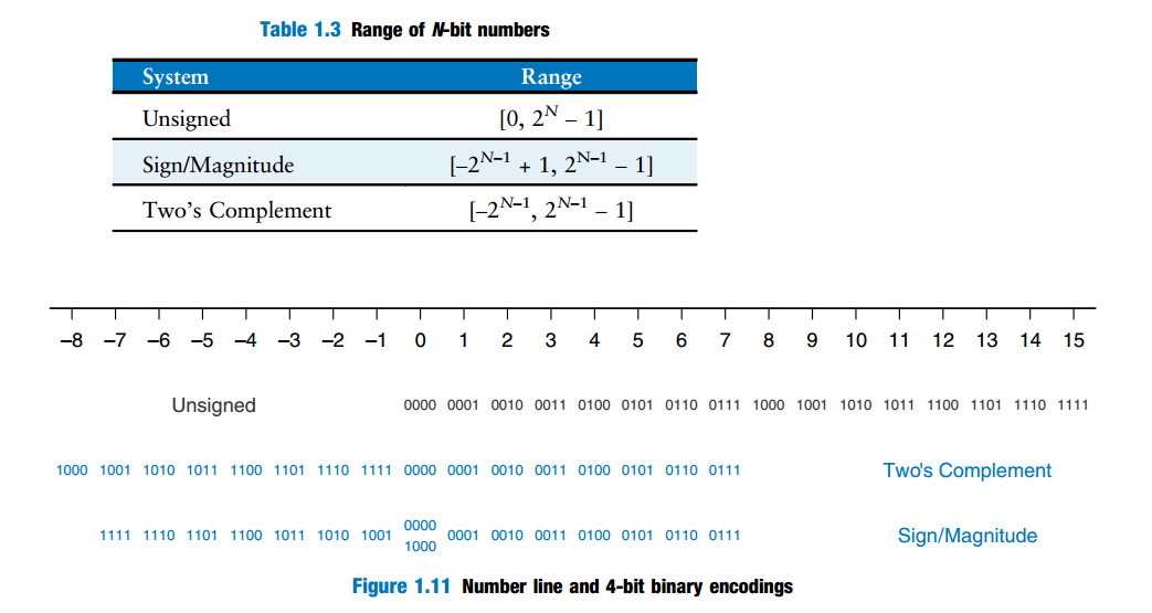
rational number
2's Complement
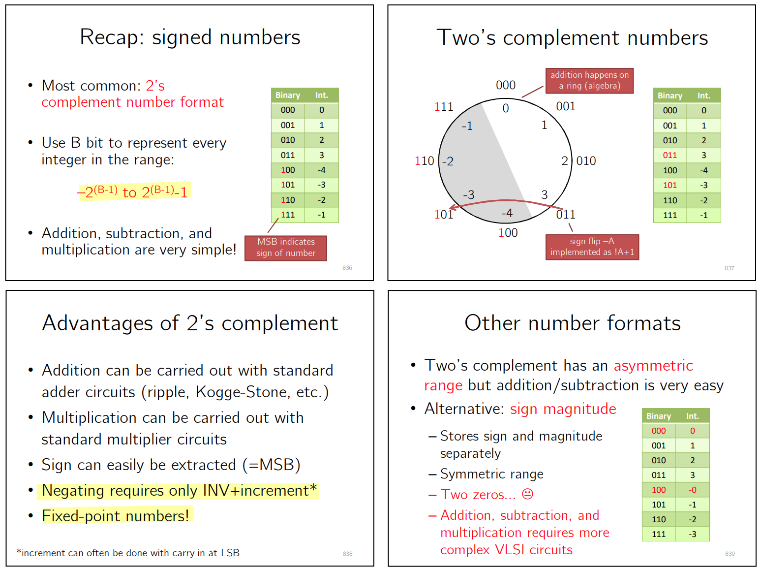
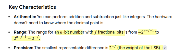
2's complement negative number
Flip all bits then Add 1
N-bit signed number \[ A = -M_{N-1}2^{N-1}+\sum_{k=0}^{N-2}M_k2^k \] Flip all bits \[\begin{align} A_{flip} &= -(1-M_{N-1})2^{N-1} +\sum_{k=0}^{N-2}(1-M_k)2^k \\ &= M_{N-1}2^{N-1}-\sum_{k=0}^{N-2}M_k2^k -2^{N-1}+\sum_{k=0}^{N-2}2^k \\ &= M_{N-1}2^{N-1}-\sum_{k=0}^{N-2}M_k2^k -1 \end{align}\]
Add 1 \[ A_- = A_{flip}+1 = M_{N-1}2^{N-1}-\sum_{k=0}^{N-2}M_k2^k = -A \]
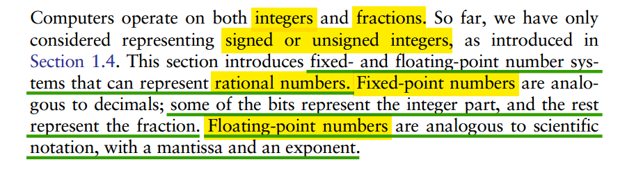
Fixed Point Number
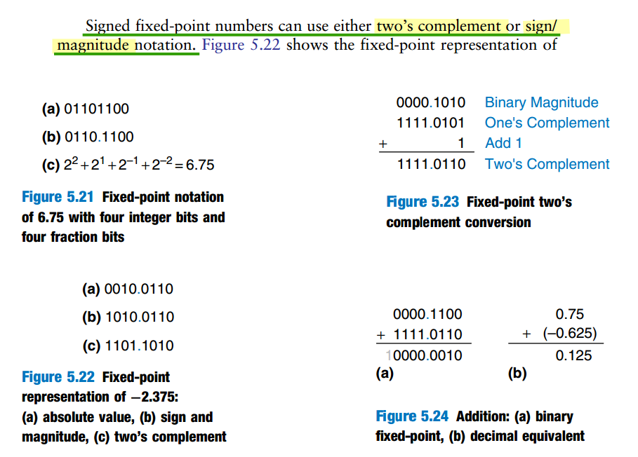
\(Q\)-Format
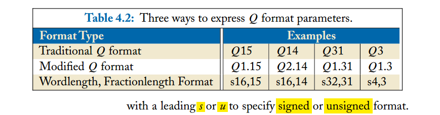
The Q notation is a way to specify the parameters of a binary fixed point number format
Q0.3 is a notation for a fixed-point binary
number format. \[
\boxed{Q0.3
=
\text{sign bit}
+
0\text{ integer bits}
+
3\text{ fractional bits}}
\]

The useful fixed-point multiplication rule is \[ Q_{F_1} \times Q_{F_2} \;\Rightarrow\; F_{\text{product}} = F_1 + F_2 \] where \(F_1\) and \(F_2\) are the numbers of fractional bits of the two operands
4-bit words are
1 | a = 0.100 -> 0100 |
Now temporarily ignore the binary point and multiply the integer bit patterns:
1 | 0100 (= 4) |
Different sources use slightly different \(Q\)-format conventions
\(Q1.3\) means that the
1 includes the sign bit. \[
Q1.3
=
\underbrace{1\text{ bit}}_{\text{sign / integer side}}
+
\underbrace{3\text{ fractional bits}}_{\text{fractional side}}
\] So it is a 4-bit two's-complement fixed-point
number:
1 | b3 . b2 b1 b0 |
Floating-point Number in IEEE 754 Format
Floating-point data in IEEE 754 Format [https://github.com/IC-Design-Lab/IC-Design/blob/main/Training/Floating-point%20data%20in%20IEEE%20754%20Format.pdf]
Rajaraman, V.. “IEEE standard for floating point numbers.” Resonance 21 (2016): 11 - 30. [https://www.ias.ac.in/article/fulltext/reso/021/01/0011-0030]
IEEE Standard for Floating-Point Arithmetic [https://www-users.cse.umn.edu/~vinals/tspot_files/phys4041/2020/IEEE%20Standard%20754-2019.pdf]
Dennis Forbes. Understanding Floating-Point Numbers [https://dennisforbes.ca/blog/features/floating_point/understanding-floating-point-numbers/]
Bevan Baas, EEC 281 - VLSI Digital Signal Processing Winter 2025 [FLOATING POINT] [FLOATING POINT <---> FIXED POINT CONVERSION]

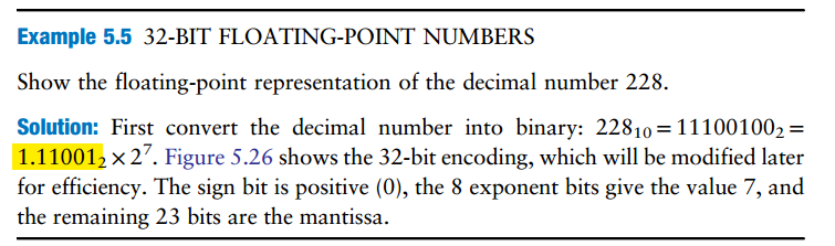
| 32-bit floating-point version 1 | store implicit leading one |  |
| 32-bit floating-point version 2 | discard implicit leading one |  |
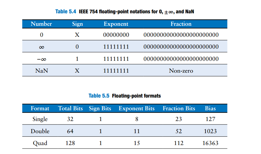
| IEEE 754 floating point notation | biased exponent | 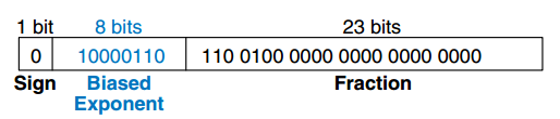 |
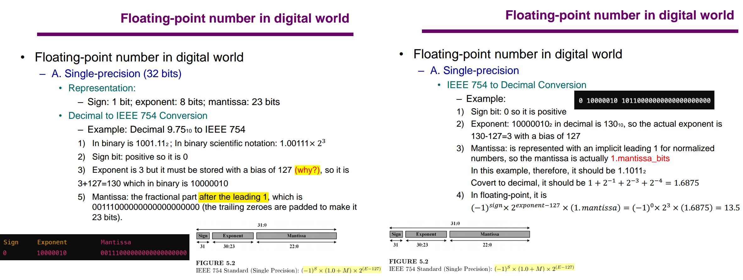
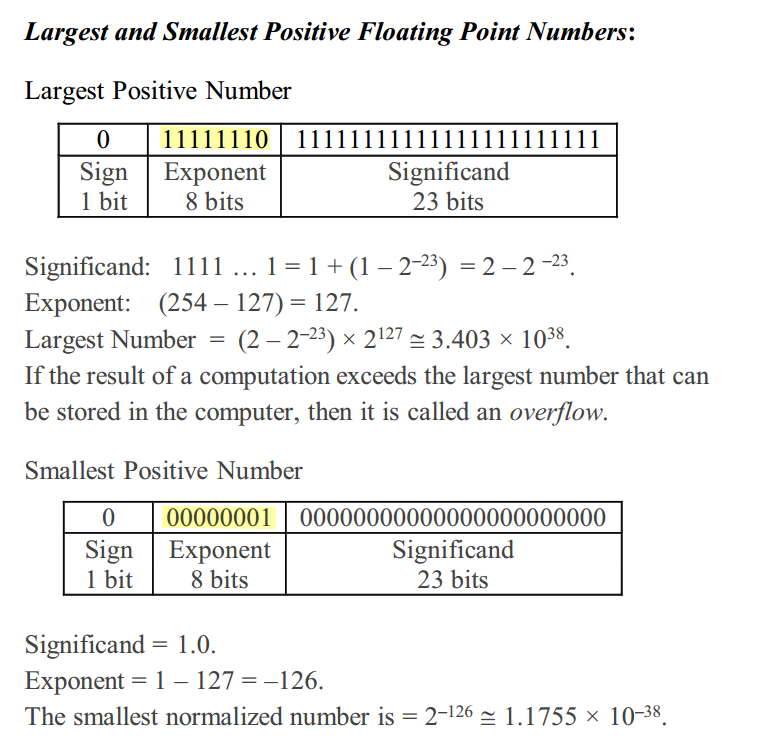 \[
\boxed{
\begin{aligned}
E=0 &: \quad \text{zero or subnormal},\\
1\le E\le254 &: \quad \text{normal finite number},\\
E=255 &: \quad \infty \text{ or NaN}.
\end{aligned}
}
\]
\[
\boxed{
\begin{aligned}
E=0 &: \quad \text{zero or subnormal},\\
1\le E\le254 &: \quad \text{normal finite number},\\
E=255 &: \quad \infty \text{ or NaN}.
\end{aligned}
}
\]
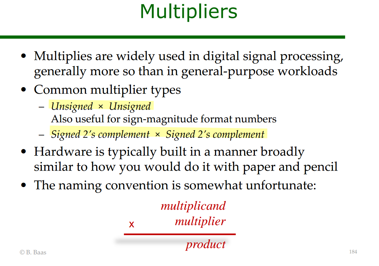
Multipliers
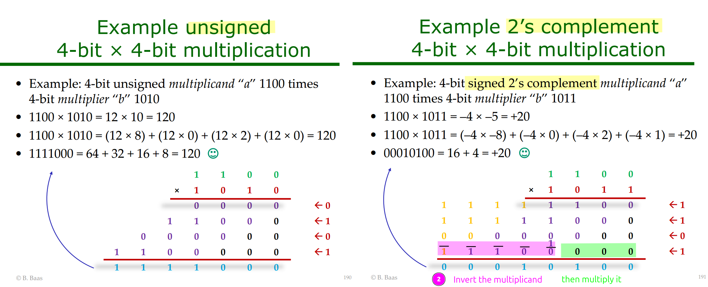
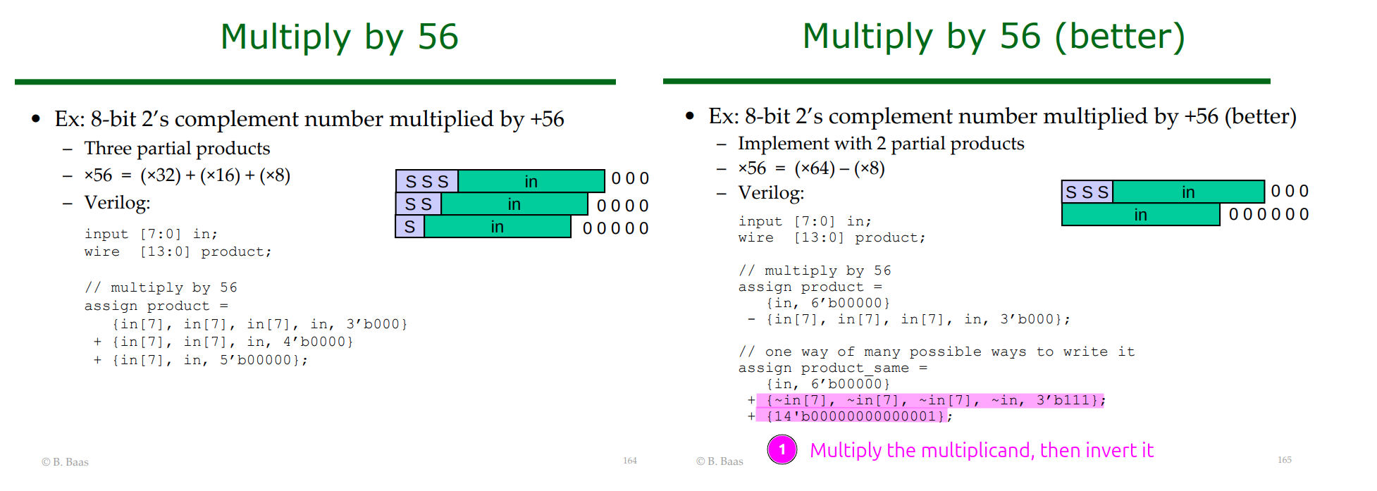
B. Baas, [HARDWARE MULTIPLIERS] [FIXED-INPUT MULTS] [MULTIPLICATION SCALING]
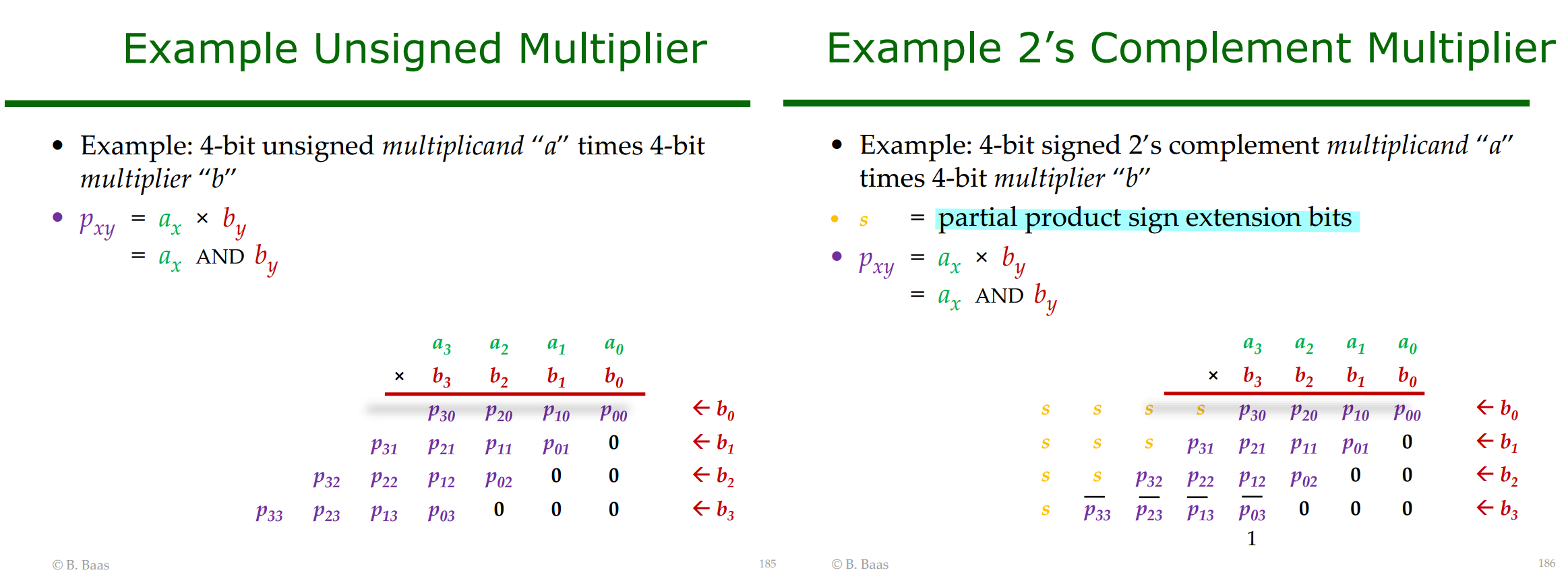
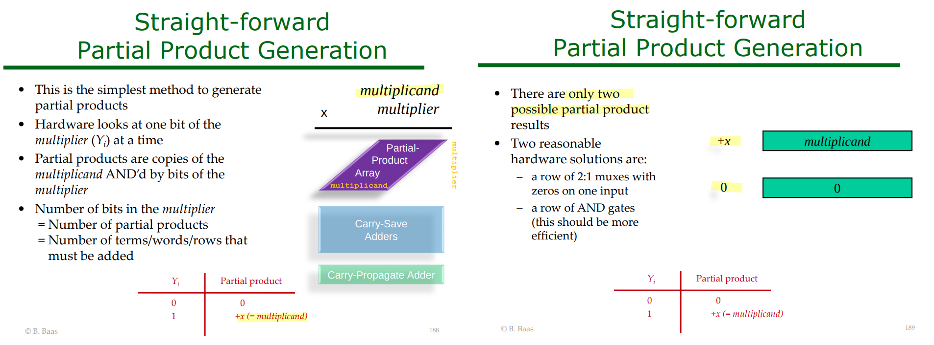
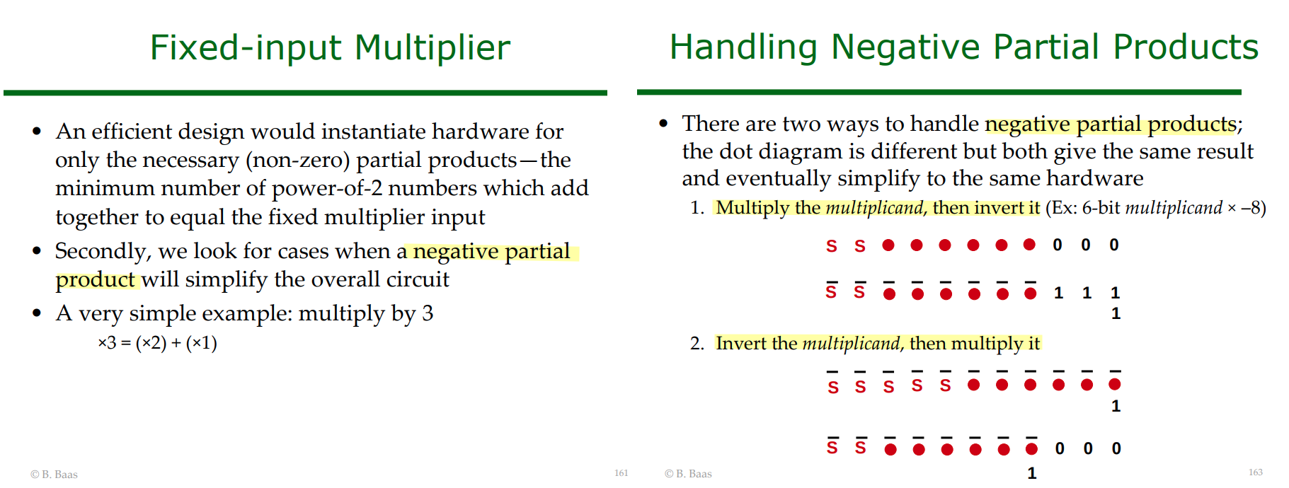
negate last partial product when multiplier[MSB]=1, i.e. multiplier is negative
- Multiply the multiplicand, then invert it
- Invert the multiplicand, then multiply it
Multiplication Scaling
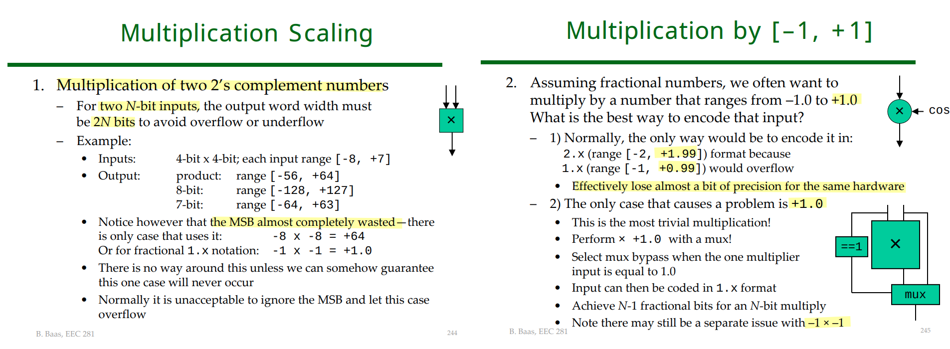
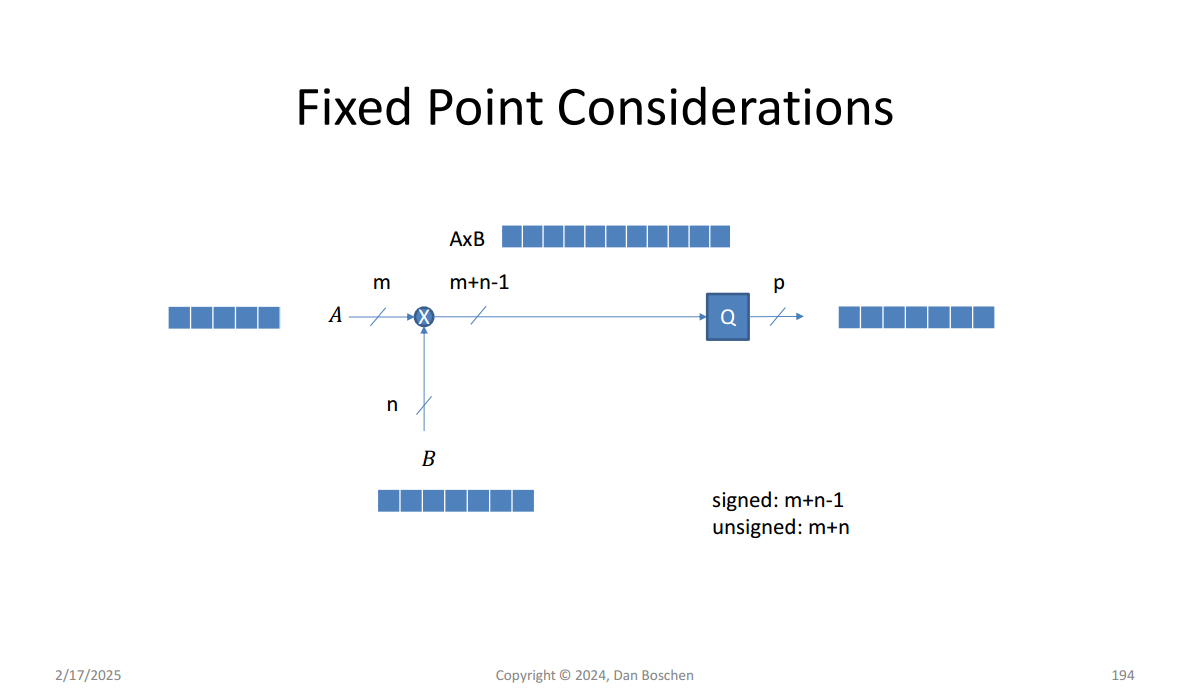
| Operands | Nominal full product width |
|---|---|
| Unsigned | \(m+n\) |
| Signed fractional | \(m+n-1\) |
For signed fractional multiplication,
\[ Q1.(m-1)\times Q1.(n-1) \rightarrow Q1.(m+n-2) \]
Therefore, the total number of bits is
\[ 1+(m+n-2)=m+n-1. \]
There is one special corner case:
\[ (-1)\times(-1)=+1 \]
but a signed fractional format such as \(Q1.(m+n-2)\) has the range
\[ -1 \le x \le 1-2^{-(m+n-2)}, \]
so it cannot represent exactly \(+1\).
Therefore:
- Normally, signed fractional multiplication requires
\[ \boxed{m+n-1\text{ bits}} \]
- To guarantee no overflow even for
\[ (-1)(-1)=+1, \]
you need
\[ \boxed{m+n\text{ bits}}. \]
Equivalently, if the operands have widths
\[ B_0+1 \quad\text{and}\quad B_1+1, \]
then the normal signed fractional product width is
\[ (B_0+1)+(B_1+1)-1 = \boxed{B_0+B_1+1}. \]
The only exception is again
\[ (-1)(-1)=+1. \]
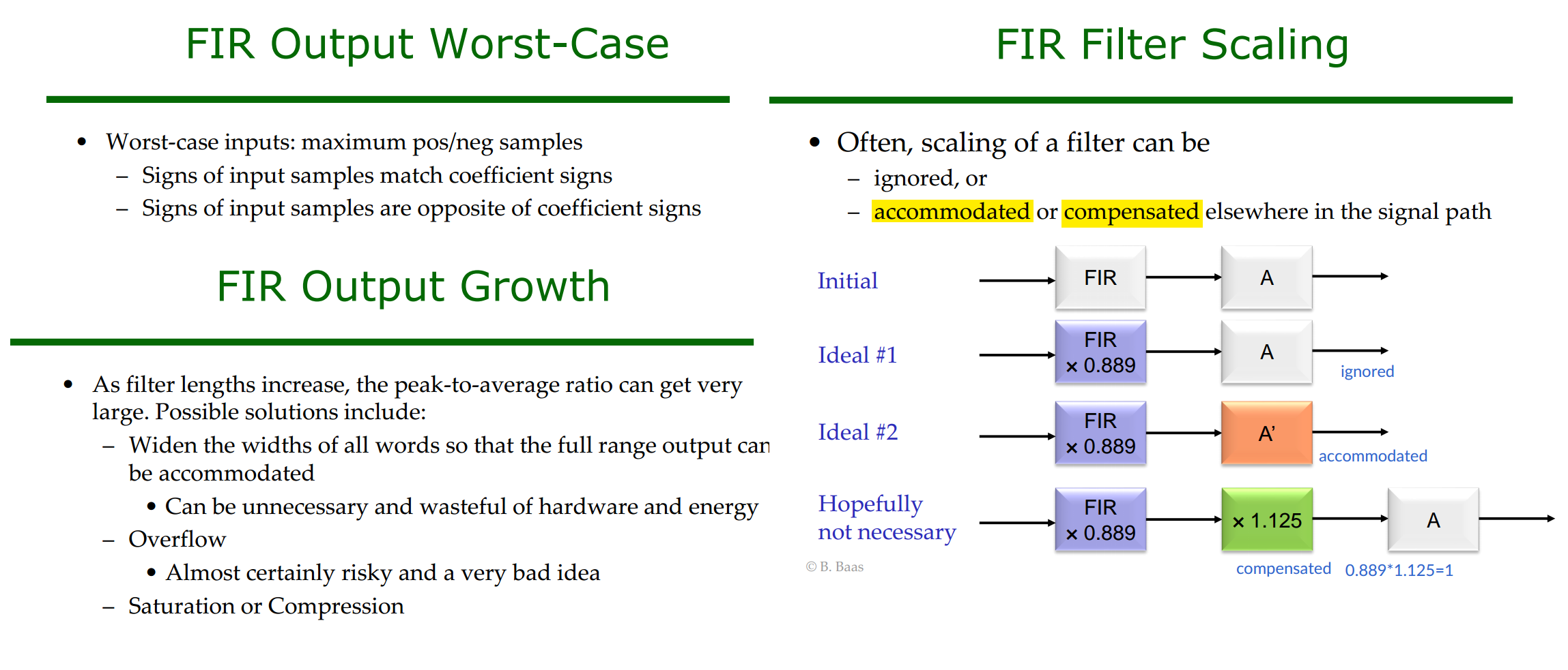
FIR Filter Scaling
Bevan Baas, EEC 281 - VLSI Digital Signal Processing Winter 2025 [FIR FILTER HARDWARE]
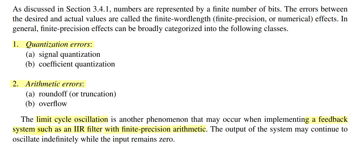
Finite-wordlength Effects
Tianshuang Qiu; Ying Guo, "7. Finite-Precision Numerical Effects in Digital Signal Processing," in Signal Processing and Data Analysis , De Gruyter, 2018, pp.236-248
Antoniou, Andreas. “Digital Signal Processing: Signals, Systems, and Filters.” (2005). [pdf]
Alan V Oppenheim, Ronald W. Schafer. Discrete-Time Signal Processing, 3rd edition
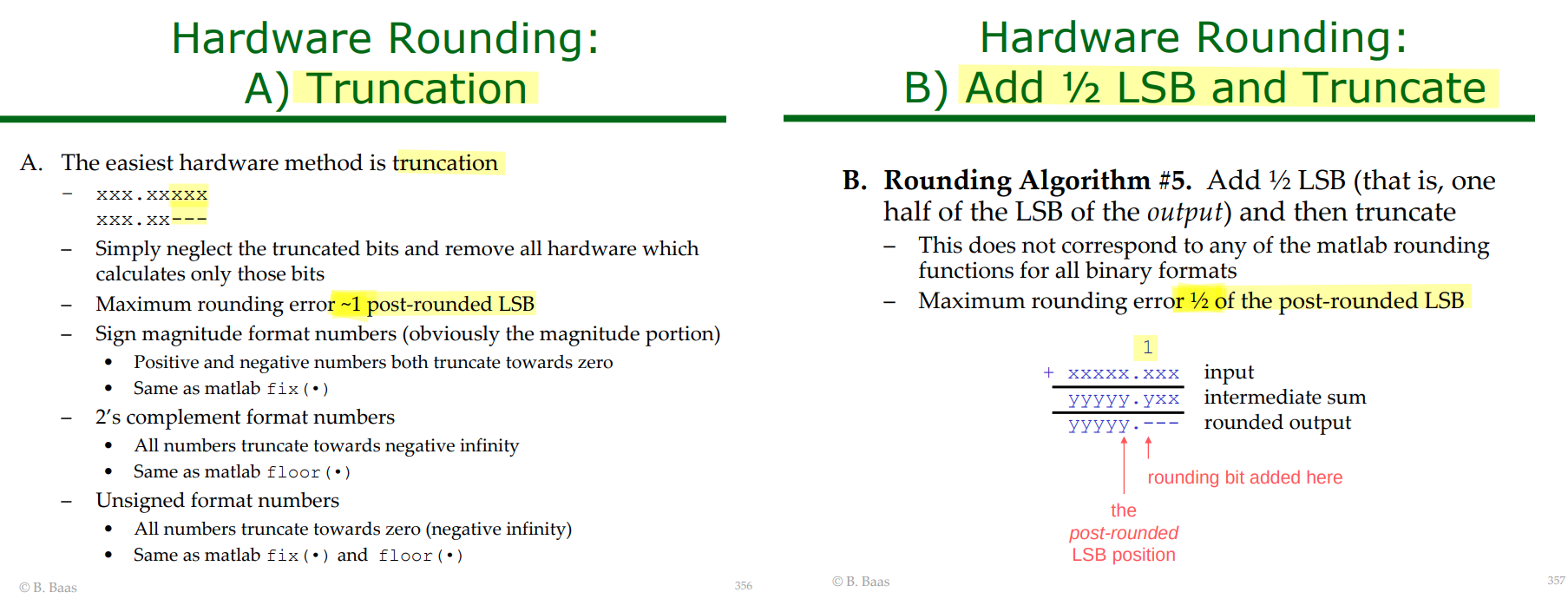
Bevan Baas, EEC 281 - VLSI Digital Signal Processing Winter 2025 [QUANTIZATION NOISE AS A FUNCTION OF WORD SIZE] [SATURATION&COMPRESSION] [ROUNDING]
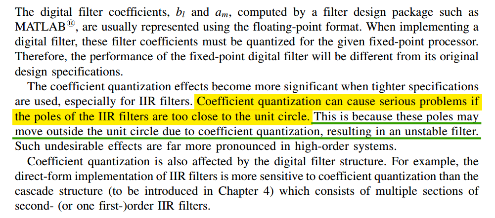
Coefficient Quantization
Roundoff Noise
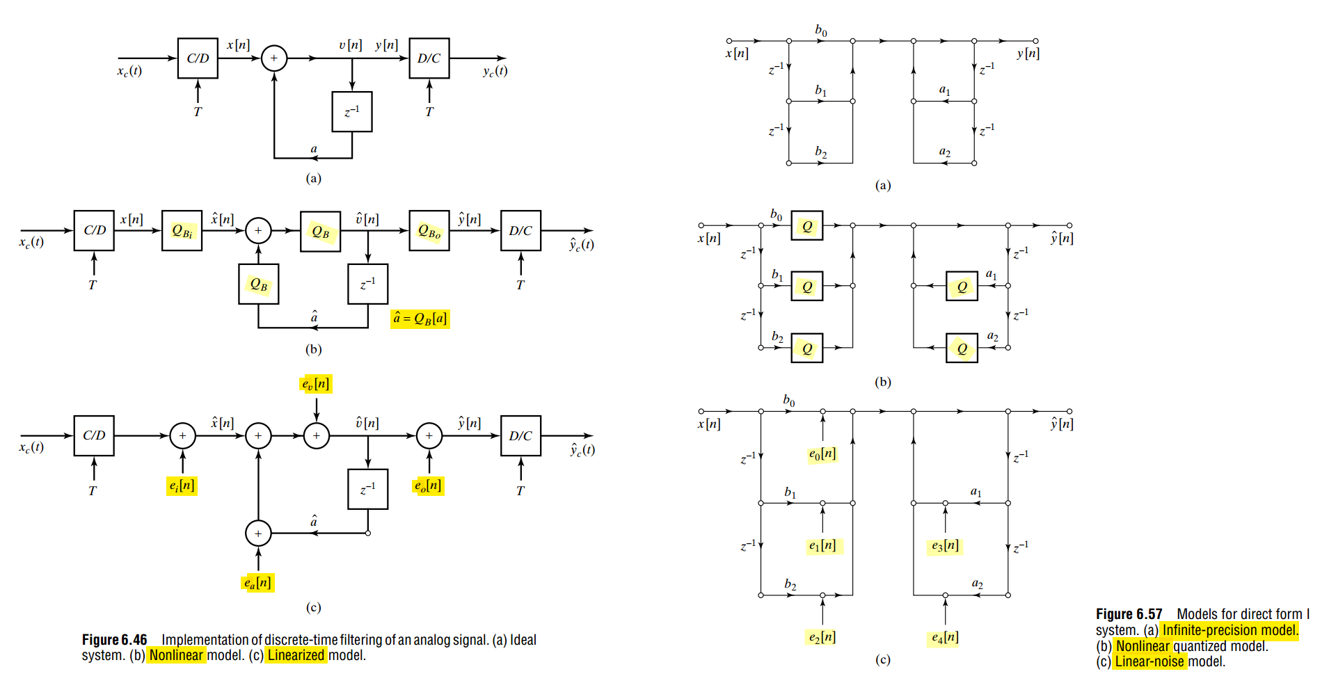
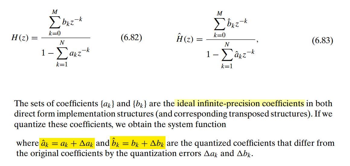
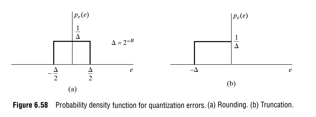
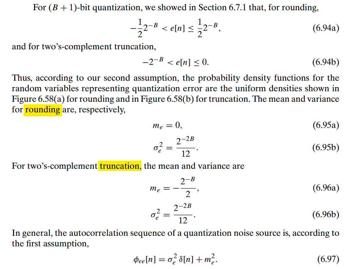
Direct-Form I (DF-I) implementation of a digital filter IIR
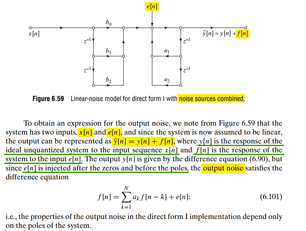
Equation (6.101) follows directly by writing the difference equation for the quantized system and subtracting the difference equation for the ideal system.
For the direct-form-I filter in Fig. 6.59, the ideal output satisfies
\[ y[n] = \sum_{k=0}^{M} b_k x[n-k] + \sum_{k=1}^{N} a_k y[n-k]. \tag{1} \]
The combined quantization noise \(e[n]\) is injected after the \(b_k\) section (zeros) and before the \(a_k\) feedback section (poles). Therefore the actual output \(\hat y[n]\) satisfies
\[ \hat y[n] = \sum_{k=0}^{M} b_k x[n-k] + \sum_{k=1}^{N} a_k \hat y[n-k] + e[n]. \tag{2} \]
The book defines
\[ \boxed{\hat y[n]=y[n]+f[n]} \]
where \(f[n]\) is the output component caused by the quantization noise
Substitute
\[ \hat y[n]=y[n]+f[n] \]
into (2):
\[ y[n]+f[n] = \sum_{k=0}^{M}b_kx[n-k] + \sum_{k=1}^{N}a_k\left(y[n-k]+f[n-k]\right) + e[n]. \]
Expand:
\[ y[n]+f[n] = \underbrace{ \sum_{k=0}^{M}b_kx[n-k] + \sum_{k=1}^{N}a_ky[n-k] }_{=\,y[n]} + \sum_{k=1}^{N}a_kf[n-k] + e[n]. \]
Using the ideal-system equation (1),
\[ y[n]+f[n] = y[n] + \sum_{k=1}^{N}a_kf[n-k] + e[n]. \]
Cancel \(y[n]\) from both sides:
\[ \boxed{ f[n] = \sum_{k=1}^{N}a_k f[n-k]+e[n] } \tag{6.101} \]
That is exactly Eq. (6.101).
Why do the \(b_k\) coefficients disappear?
This is the important point.
The signal path is
\[ x[n] \rightarrow \underbrace{B(z)}_{\text{zeros}} \rightarrow \boxed{+\,e[n]} \rightarrow \underbrace{\frac{1}{A(z)}}_{\text{poles}} \rightarrow \hat y[n]. \]
The noise is inserted after \(B(z)\), so it never passes through the zeros. It only passes through the all-pole feedback section.
In the \(z\)-domain, Eq. (6.101) gives
\[ F(z) = \sum_{k=1}^{N}a_kz^{-k}F(z)+E(z). \]
Thus,
\[ F(z) \left( 1-\sum_{k=1}^{N}a_kz^{-k} \right) = E(z), \]
and therefore
\[ \boxed{ \frac{F(z)}{E(z)} = \frac{1} {1-\displaystyle\sum_{k=1}^{N}a_kz^{-k}} } \]
So the output quantization-noise transfer function contains only the poles, which is what the sentence immediately after (6.101) means.
For the second-order example in the figure,
\[ \boxed{ f[n]=a_1f[n-1]+a_2f[n-2]+e[n]. } \]
The coefficients \(b_0,b_1,b_2\) have no effect on \(f[n]\) because \(e[n]\) is injected after that part of the filter.
Limit Cycles in feedback system
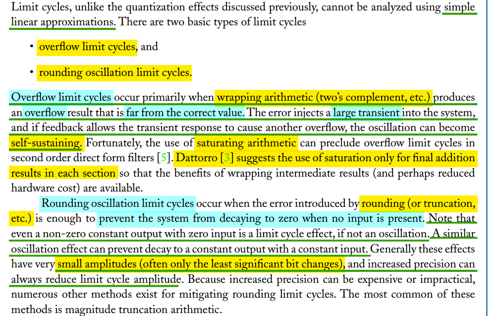
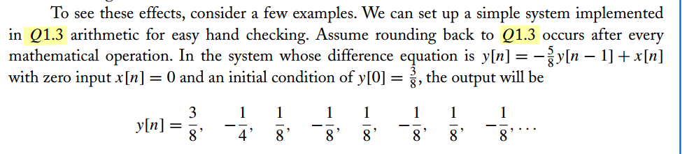
Limit Cycles Owing to Round-off & Truncation
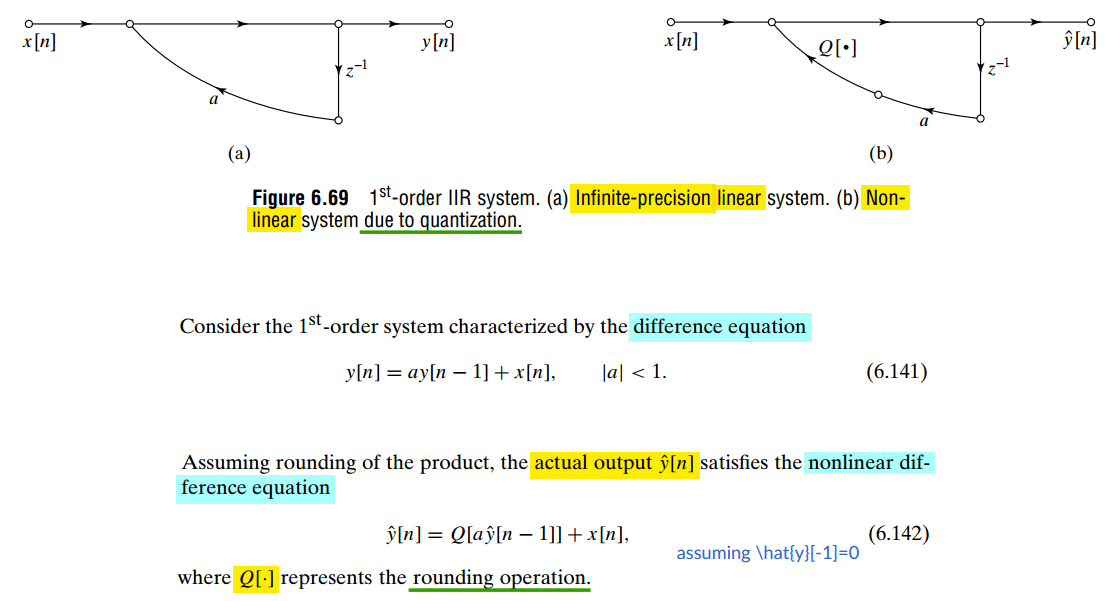
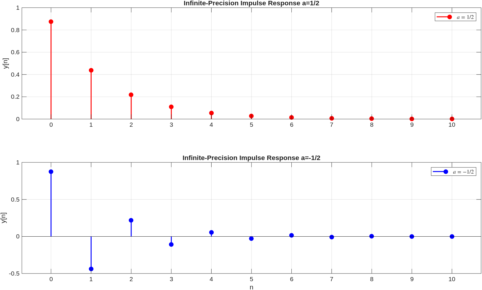
For infinite-precision linear system \(y[n] = a y[n-1] + x[n],\)
with zero initial condition \(y[-1]=0\), the impulse response is \[ y[n] = \frac{7}{8} a^n u[n] \] because after the impulse at \(n=0\), we have \(x[n]=0\) for all \(n\ge 1\).
For nonlinear system \(\hat{y}[n] = Q[a \hat{y}[n-1]] + x[n],\)
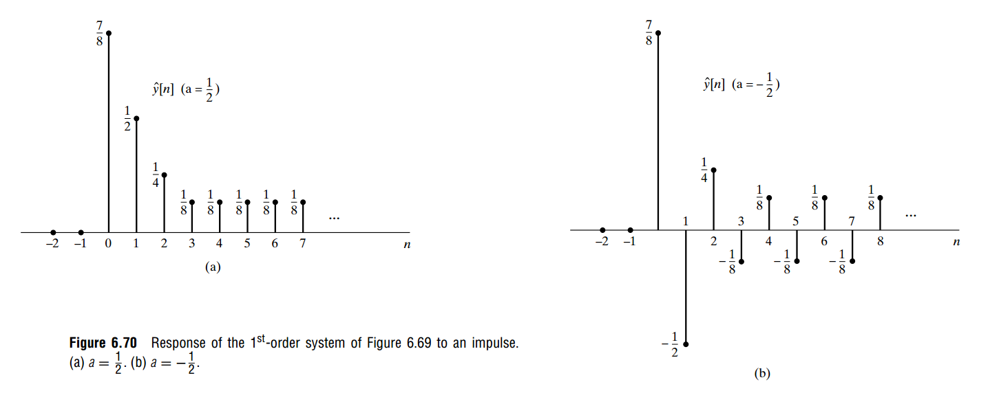
The nonzero steady oscillation or constant value is created entirely by the rounding operation (nonlinear) \(Q[\cdot]\)
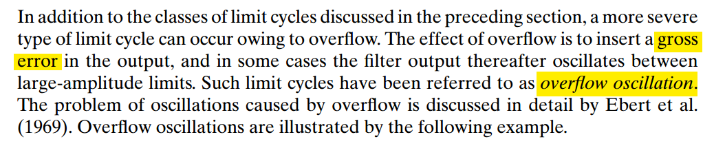
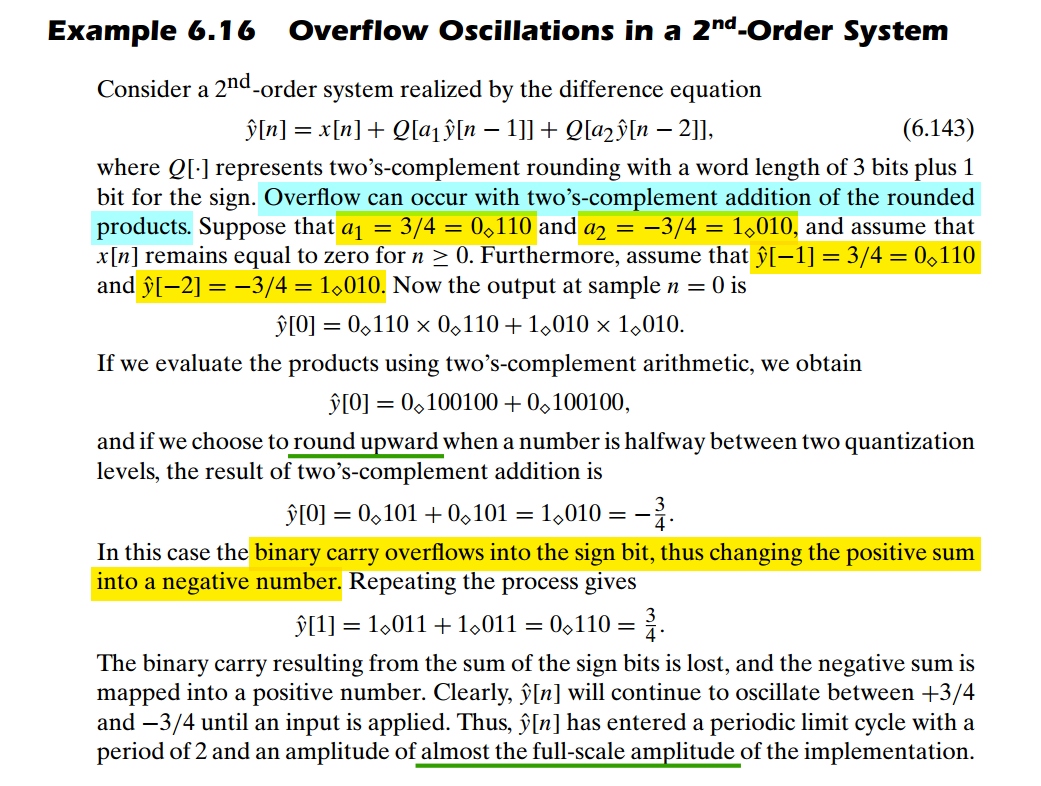
Limit Cycles Owing to Overflow
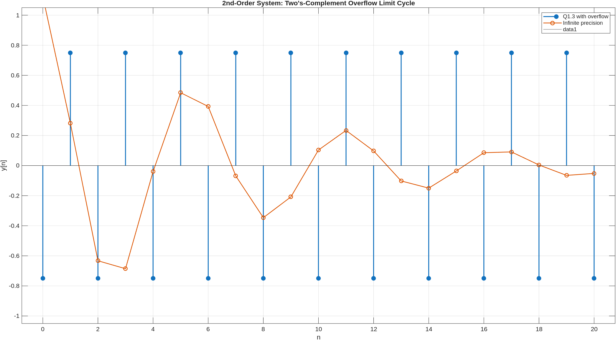
1 | %% Parameters |
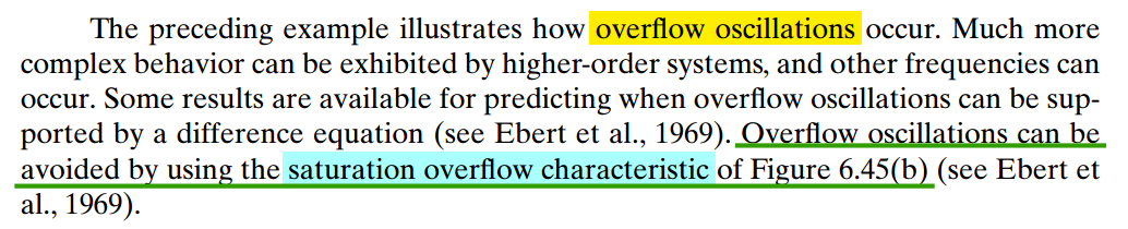
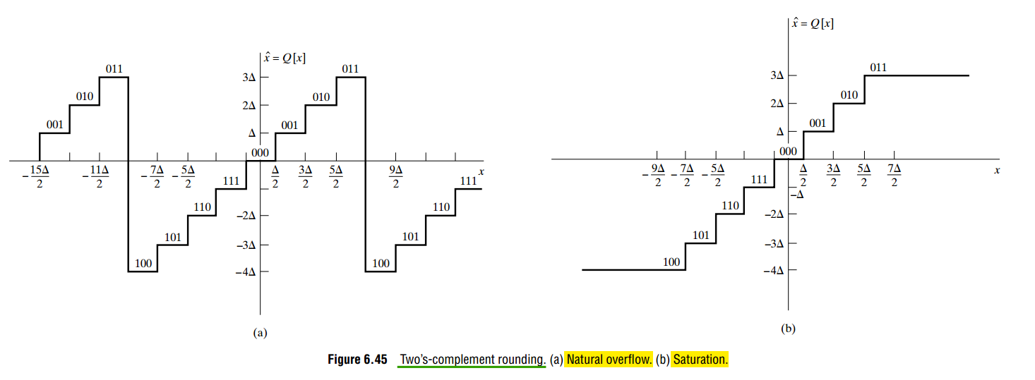
1 | //------------------------------------------------------------------------- |
Avoiding Limit Cycles
The suppression of limit cycles is a broad topic with all the complexity to be expected in a nonlinear system behavior.
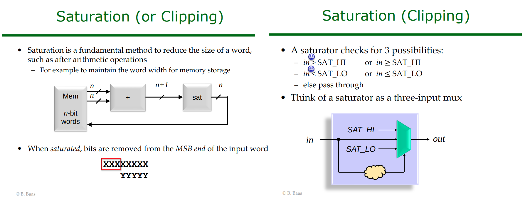
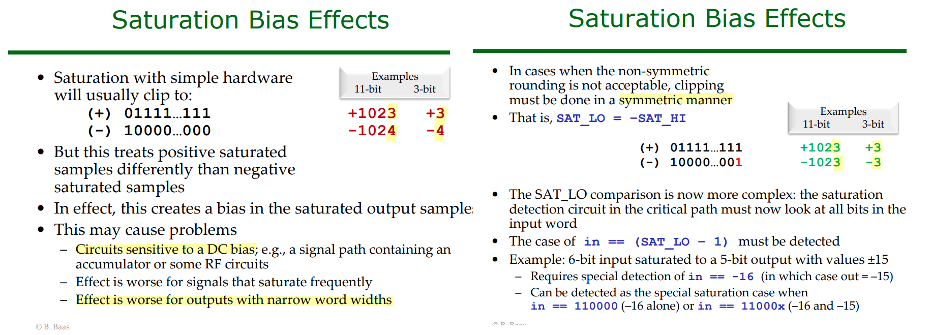
The most basic tools of saturation arithmetic and magnitude truncation — rounding rounds toward zero

Saturation Arithmetic & Scaling of Signals
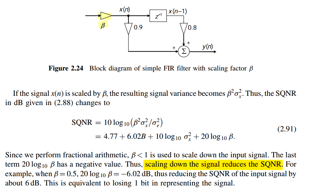
Saturation arithmetic prevents overflow by clipping the results to a maximum value
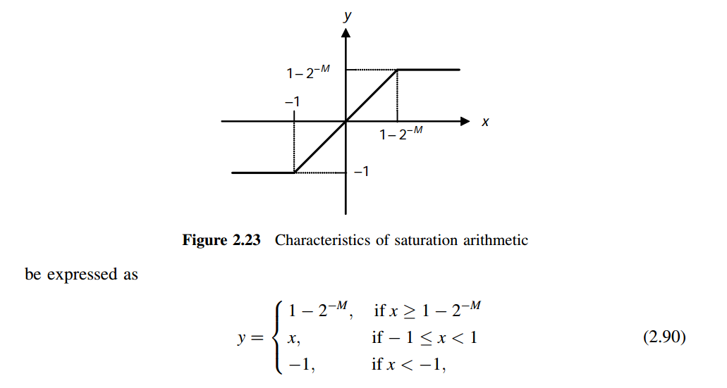
The most effective technique in preventing overflow is by scaling down the signal
Saturation Bias Effects
FFE implemented in DSP
M. A. Kossel et al., "8.3 An 8b DAC-Based SST TX Using Metal Gate Resistors with 1.4pJ/b Efficiency at 112Gb/s PAM-4 and 8-Tap FFE in 7nm CMOS," 2021 IEEE International Solid-State Circuits Conference (ISSCC), San Francisco, CA, USA, 2021, pp. 130-132 [https://sci-hub.ru/10.1109/ISSCC42613.2021.9365784]
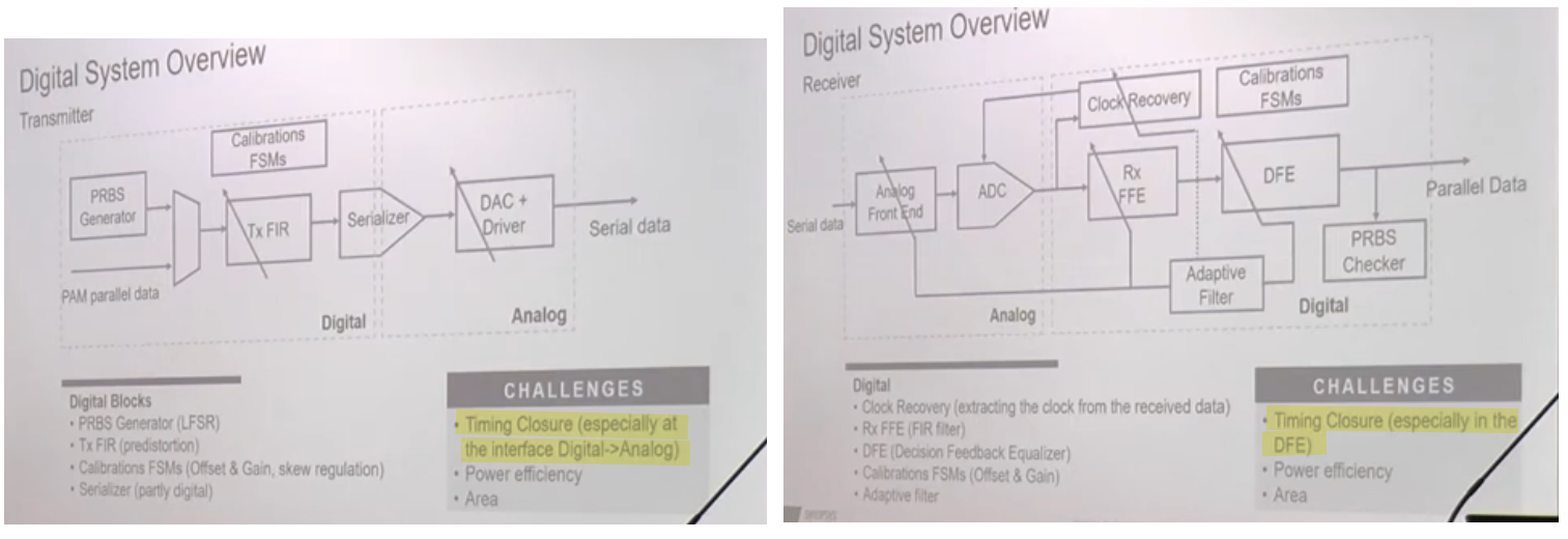
DFE in digital
Synopsys Italia, Tech Talk: Introduction to DSP-based SerDes [https://youtu.be/puEP0DlVZGI]
Chen, Kuan-Chang (2022) Energy-Efficient Receiver Design for High-Speed Interconnects. Dissertation (Ph.D.), California Institute of Technology. [https://thesis.library.caltech.edu/14318/9/chen_kuan-chang_2022_thesis_final.pdf]
Parallel implementation
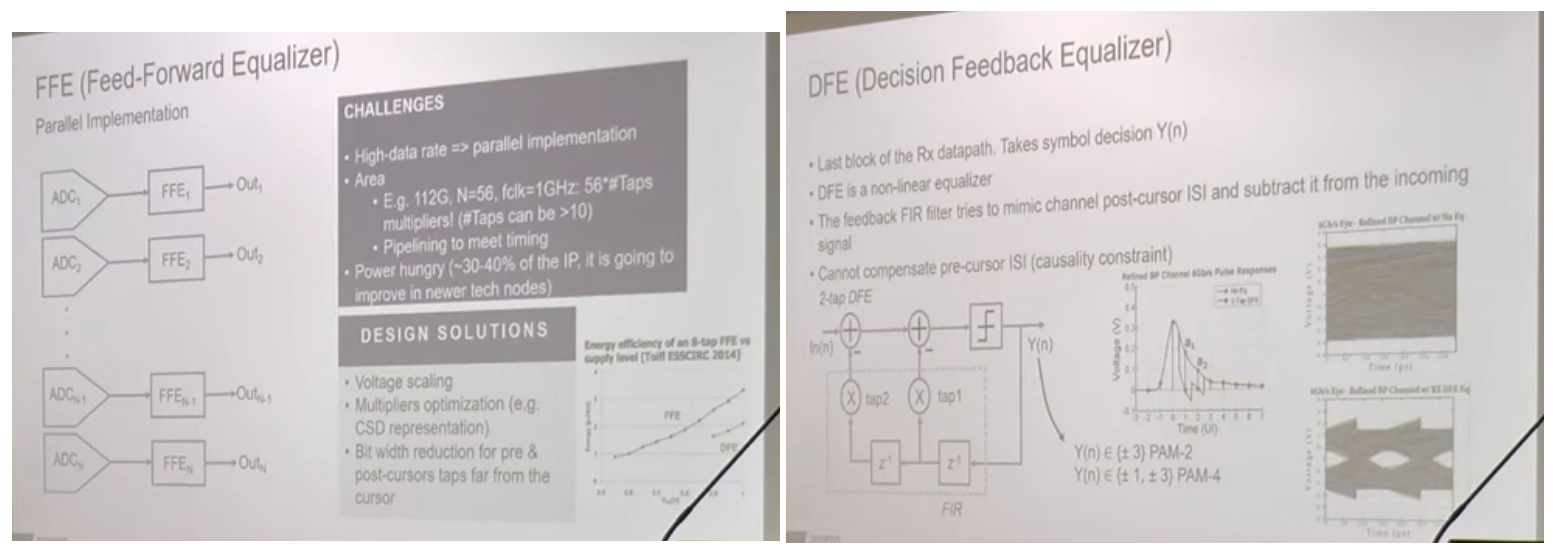
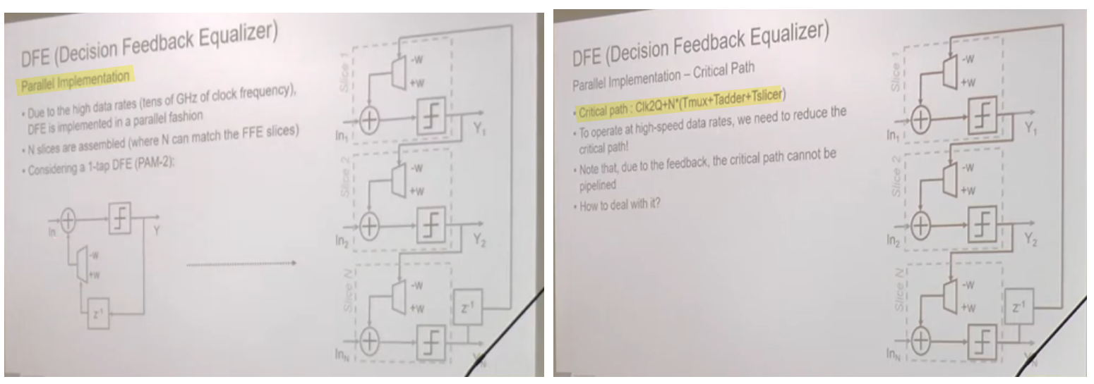
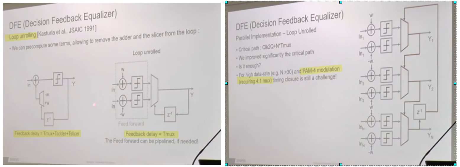
Loop-Unrolling DFE
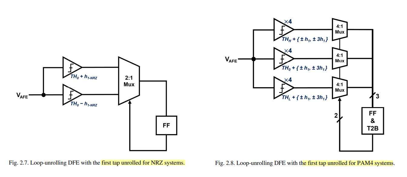
Corresponding to the three distinct voltage thresholds in the PAM4 systems, it would need 12 slicers, 3 multiplexers, and one thermometer-to-binary decoder in each deserialized data path, even if only one tap of the DFE is unrolled
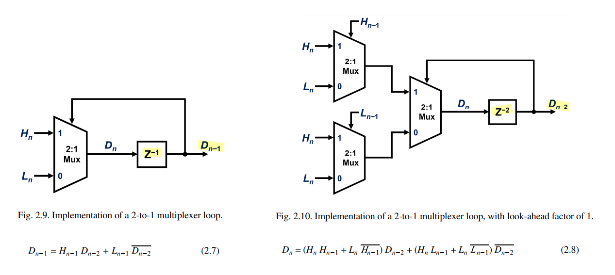
Look-Ahead Multiplexing DFE
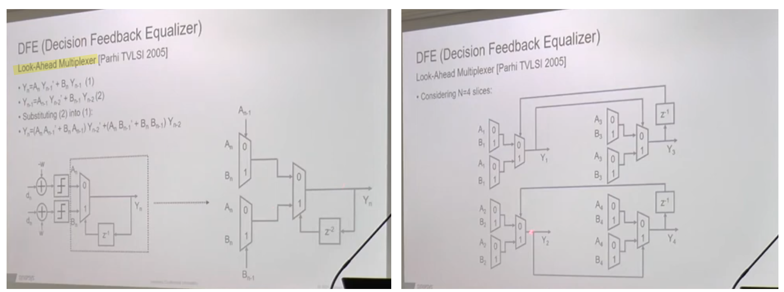
The look-ahead multiplexing technique brings the key benefit that the timing constraint can be significantly relaxed, as the iteration bound is doubled at the expense of extra hardware
MASH 1-1-1 in Verilog
MASH-1-1-1 Noise-Shaping Truncator (DLF → DAC) [https://github.com/raytroop/dsmwk]
Digital block between a 20-bit digital loop filter (DLF) output and an 8-bit DAC input. The 12 truncated LSBs are pushed through a MASH-1-1-1 delta-sigma modulator so the truncation error is 3rd-order noise-shaped instead of lost:
1 | dac(z) = dlf(z)/2^12 - (1 - z^-1)^3 · q(z) (× z^-1 latency) |
where e3 is the stage-3 accumulator residue in raw
20-bit-LSB counts (0…4095, quantizer step 2¹²) and q is the
same error referred to the 8-bit output grid — the unit-step
quantization noise of the effective 1-LSB₈ quantizer.
dac(z) = dlfMSB8 (z)/212 + dlfLSB12 (z)/212+ q(z) · (1 - z-1)3 = dlf(z)/212 + q(z) · (1 - z-1)3
1 | dlf_in[19:12] ─────────────────────────────────┐ |
flowchart LR
    IN["dlf_in<br/>20 bits"] -->|"upper 8 bits"| XMSB["x_msb<br/>coarse value"]
    IN -->|"lower 12 bits"| A1["Stage 1<br/>acc1 + x_frac"]

    R1[("acc1<br/>register")] --> A1
    A1 -->|"residue r1"| R1
    A1 -->|"r1"| A2["Stage 2<br/>acc2 + r1"]
    A1 -->|"carry c1"| NC["Noise cancellation<br/>c1 + c2 − c2_d1<br/>+ c3 − 2c3_d1 + c3_d2"]

    R2[("acc2<br/>register")] --> A2
    A2 -->|"residue r2"| R2
    A2 -->|"r2"| A3["Stage 3<br/>acc3 + r2"]
    A2 -->|"carry c2"| NC
    A2 -->|"c2"| C2D1[("c2_d1<br/>z⁻¹")]
    C2D1 -->|"−c2_d1"| NC

    R3[("acc3<br/>register")] --> A3
    A3 -->|"residue r3"| R3
    A3 -->|"carry c3"| NC
    A3 -->|"c3"| C3D1[("c3_d1<br/>z⁻¹")]
    C3D1 -->|"−2c3_d1"| NC
    C3D1 --> C3D2[("c3_d2<br/>z⁻²")]
    C3D2 -->|"+c3_d2"| NC

    NC -->|"signed correction y<br/>−3…+4"| ADD["x_msb + y"]
    XMSB --> ADD
    ADD --> SAT["Clamp to 0…255"]
    SAT --> OUTREG[("Output register")]
OUTREG --> OUT["dac_out<br/>8 bits"]| Branch | Expression | Range |
|---|---|---|
| stage 1 | c1 |
{0, 1} |
| stage 2 | (1−z⁻¹)·c2 = c2 − c2_d1 |
{−1, 0, +1} |
| stage 3 | (1−z⁻¹)²·c3 = c3 − 2·c3_d1 + c3_d2 |
[−2, +2] |
| total | y |
[−3, +4] |
1 | wire signed [5:0] y = |
Each carry is a bare bit {0,1}. {5'b0, c1}
zero-extends it to 6 bits (value unchanged), and
$signed(...) marks it for signed arithmetic. The term
{4'b0, c3_d1, 1'b0} is c3_d1 with a zero
appended — a shift-left-by-1, i.e. 2·c3_d1 (value 0 or 2) —
so the multiply costs nothing.
The reachable values of y and their actual bit
patterns:
| value | y[5:0] |
value | y[5:0] |
|
|---|---|---|---|---|
| +4 | 000100 |
0 | 000000 |
|
| +3 | 000011 |
−1 | 111111 |
|
| +2 | 000010 |
−2 | 111110 |
|
| +1 | 000001 |
−3 | 111101 |
Worked example:
c1=0, c2=0, c2_d1=1, c3=0, c3_d1=1, c3_d2=0 →
y = 0 + (0−1) + (0−2+0) = −3 → 111101.
clamp [-3, 259] to [0, 255]
For msb ∈ [3, 251], x_msb + y never leaves
[0,255], the mux always takes the pass-through leg, and
dac_sat ≡ dac_sum bit-for-bit.
1 | //------------------------------------------------------------------------- |
In a locked PLL the DLF integrator sits mid-range and the clamp never fires — cost: zero. It engages only during acquisition/slew, where noise is irrelevant and its job is exactly right: drive the DAC monotonically to the rail without wrapping
overall ENOB calculation
1 | SNR = P_sig / (P_q,in + P_dsm) (powers add — sources are independent) |
with everything in the same units (LSB₈² is convenient) and — critically — both noise terms integrated in-band only (0 … f_bw, i.e. what survives the analog filter):
| Term | Expression (LSB₈², fs = f_clk) |
|---|---|
| Signal (full-scale sine convention) | P_sig = FS²/8 = 256²/8 = 8192 |
| DSM shaped noise, in-band | P_dsm = (1/12)·(π⁶/7)·OSR⁻⁷ |
| Input quantization noise, in-band | P_q,in = (2⁻¹²)²/12 · κ |
Sanity check at OSR = 50 (static input, κ=1):
P_q,in = 4.97e-9, P_dsm = 1.47e-11 → SNR =
122.1 dB → ENOB = 19.98 — the DSM costs only 0.13 dB
against the ideal 20.00. At OSR = 10: DSM dominates, ENOB = 16.1
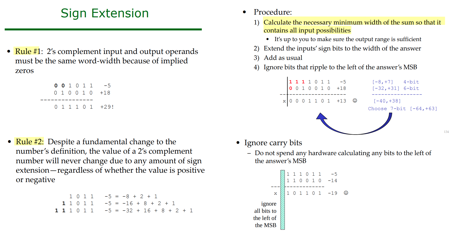
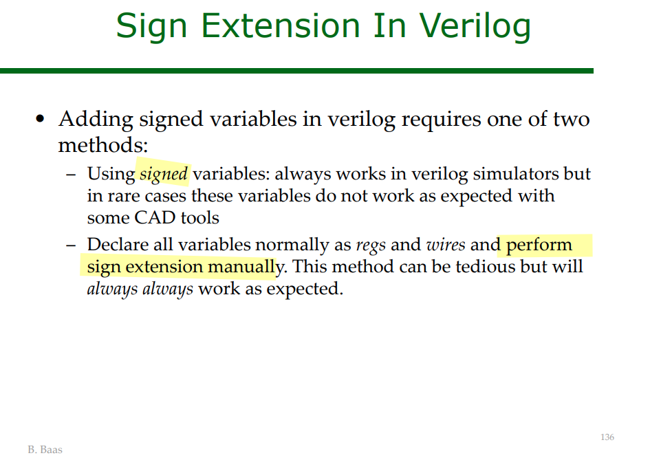
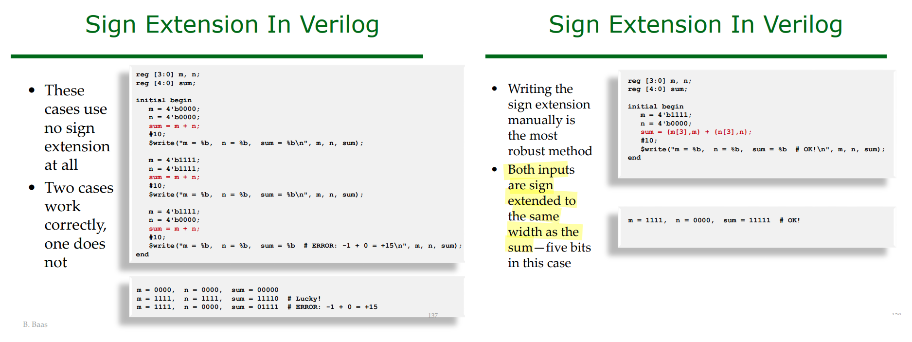
Sign Extension In Verilog
[https://www.ece.ucdavis.edu/~bbaas/281/notes/Handout.sign.extension.pdf]
One-Hot and Thermometer (Unary) codes
An N-bit binary input represents \(2^{N}\) unique values (from 0 to \(2^N - 1\))
Converting this input requires a \(2^{N}\)-bit width for One-Hot encoding, but only a \((2^N - 1)\)-bit width for Thermometer Code, as the value zero is represented by all zeros
| Decimal | Binary (\(N=3\)) | One-Hot (\(2^3 = 8\)) bits) | Thermometer (\(2^3 - 1 = 7\)) bits) |
|---|---|---|---|
| 0 | 000 |
00000001 |
0000000 |
| 1 | 001 |
00000010 |
0000001 |
| 2 | 010 |
00000100 |
0000011 |
| 3 | 011 |
00001000 |
0000111 |
| 4 | 100 |
00010000 |
0001111 |
| 5 | 101 |
00100000 |
0011111 |
| 6 | 110 |
01000000 |
0111111 |
| 7 | 111 |
10000000 |
1111111 |
RTL module
MakerCode RTL Challenge [https://github.com/Weiyet/MakerCode_RTLChallenge]
decimation_filter
Filter Equation
1 | filtered[n] = (1*x[n] + 3*x[n-1] + 3*x[n-2] + 1*x[n-3]) / 8 |
1 | iverilog -g2012 -o sim.vvp solution.sv tb.sv |
1 | module decimation_filter #( |
Line 34 uses non-blocking assignment:
1 | x1 <= data_in; // line 34: scheduled, NOT applied yet |
Non-blocking assignments don't take effect until the end of the current time step (after all the blocking statements in the block have run). So at line 37:
x1still holds its previous value — i.e. the sample from the lastdata_valid_incycle, which isx[n-1].data_inis the current sample,x[n].
They are different values. That's deliberate and necessary for the FIR math to be correct:
1 | filtered = 1*x[n] + 3*x[n-1] + 3*x[n-2] + 1*x[n-3] |
| Symbol | Value at line 37 | Filter tap |
|---|---|---|
data_in |
x[n] (current) | coeff 1 |
x1 |
x[n-1] | coeff 3 |
x2 |
x[n-2] | coeff 3 |
x3 |
x[n-3] | coeff 1 |

gray-code
1 | function automatic logic [3:0] bin2gray(input logic [3:0] bin); |
1 | function automatic logic [3:0] bin2gray(input logic [3:0] bin); |
reference
Padgett, Wayne T. and David V. Anderson. "Fixed-Point Signal Processing." Synthesis Lectures on Signal Processing (2009).
Alan V Oppenheim, Ronald W. Schafer. Discrete-Time Signal Processing, 3rd edition
Jabbour, Chadi, etc.. "Digitally enhanced mixed signal systems." IEEE International Symposium on Circuits and Systems (ISCAS). 2019.
Sen M. Kuo. Real-Time Digital Signal Processing: Fundamentals, Implementations and Applications, 3rd Edition. John Wiley & Sons 2013 [pdf]
Taylor, Fred. Digital filters: principles and applications with MATLAB. John Wiley & Sons, 2011
D. Markovic and R. W. Brodersen, DSP Architecture Design Essentials, Springer, 2012.
X. Yang, Integrated Circuit Design: IC Design Flow and Project-Based Learning, 1st edition. Boca Raton: CRC Press, 2024 [repo]
Bevan Baas, EEC281 VLSI Digital Signal Processing, [https://www.ece.ucdavis.edu/~bbaas/281/]
Mark Horowitz. EE371: Advanced VLSI Circuit Design Spring 2006-2007 [https://web.stanford.edu/class/archive/ee/ee371/ee371.1066/]
Tinoosh Mohsenin. CMPE 691: Digital Signal Processing Hardware Implementation [https://userpages.cs.umbc.edu/tinoosh/cmpe691/]
Keshab K. Parhi [http://www.ece.umn.edu/users/parhi/]
謝秉璇. 2019 積體電路設計導論 [link]
Jason Sachs. Understanding and Preventing Overflow (I Had Too Much to Add Last Night) [https://www.embeddedrelated.com/showarticle/532.php]
—. Round Round Get Around: Why Fixed-Point Right-Shifts Are Just Fine [https://www.embeddedrelated.com/showarticle/1015.php]
—. How to Build a Fixed-Point PI Controller That Just Works: Part I [https://www.embeddedrelated.com/showarticle/121.php]
—. How to Build a Fixed-Point PI Controller That Just Works: Part II [https://www.embeddedrelated.com/showarticle/123.php]
AHMED SHAHEIN, Fixed-Point Simulation in GNU Octave—Without MATLAB [https://www.dsprelated.com/showarticle/1786.php]
A. Antoniou, "On the roots of digital signal processing. Part I," in IEEE Circuits and Systems Magazine, vol. 7, no. 1, pp. 8-18, First Quarter 2007
—, "Feature - On the roots of digital signal processing - Part II," in IEEE Circuits and Systems Magazine, vol. 7, no. 4, pp. 8-19, Fourth Quarter 2007
Hideo Okawara's Mixed Signal Lecture Series [https://tomverbeure.github.io/2024/01/06/Hideo-Okawara-Mixed-Signal-Lecture-Series.html]
Jeffrey Walling, DSP to ASIC Block [https://youtube.com/playlist?list=PLP4ZmM6GPueNEdnLhgkdr8_X8dSizUwMs]
Abdur Rafae Haqqani, Embedded Systems / FPGA Blogs On Request Rounding, dither and saturation when you cut word width in FPGA DSP. [https://rafae1130.github.io/posts/on-request/fractions-in-fpga.html]