Fixed-Point Signal Processing

Posted on 2025-11-11 Edited on 2026-11-14 In dsp

why fixed-point arithmetic?

Because the dynamic range of the incoming physical signal is tightly controlled by an Analog Front End (AFE) using Automatic Gain Control (AGC), a massive floating-point dynamic range isn't necessary

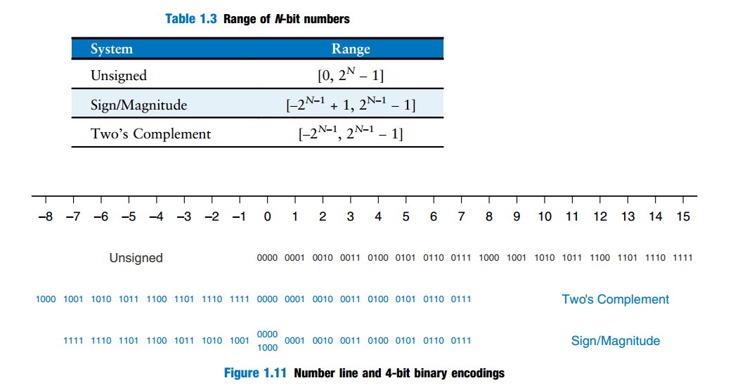
N-bit number

Harris, David Money, and Sarah L. Harris. Digital Design and Computer Architecture. 2nd ed. Morgan Kaufmann, 2013. [pdf]

integers

rational number

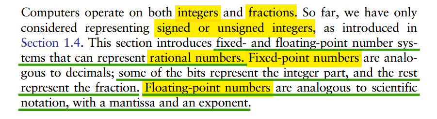
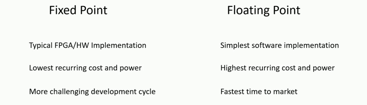
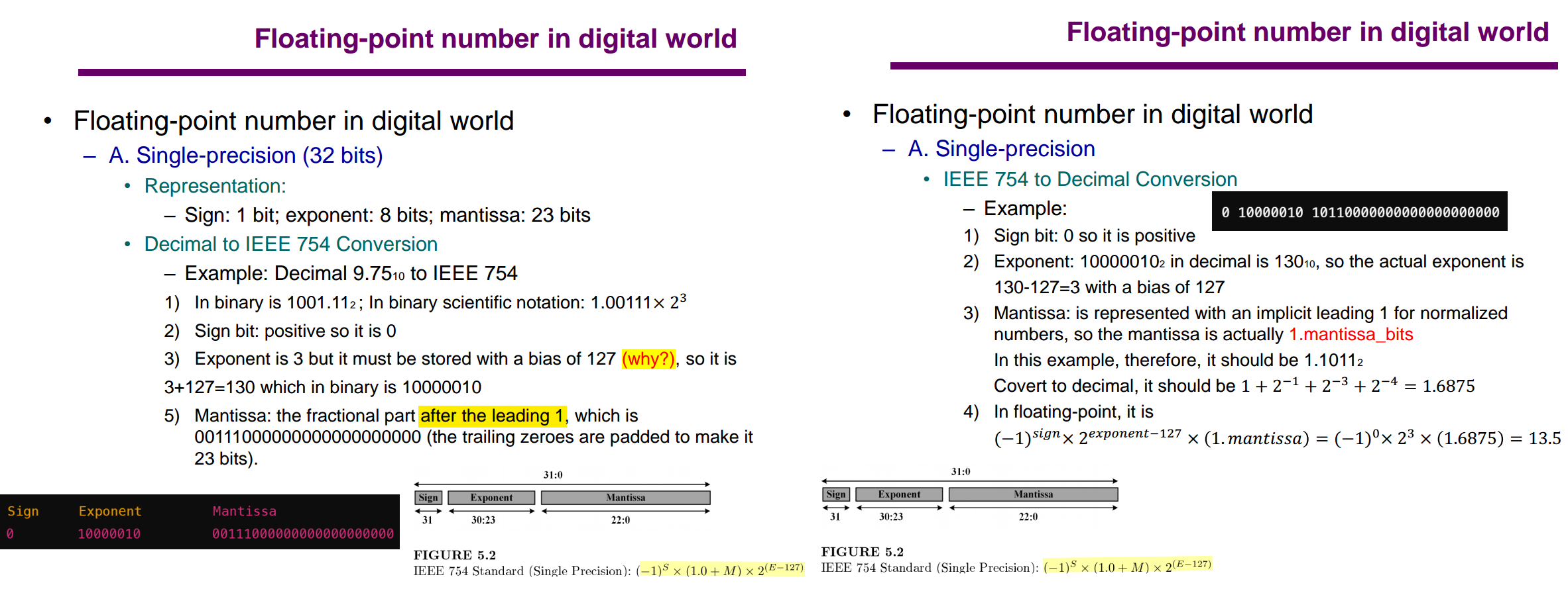
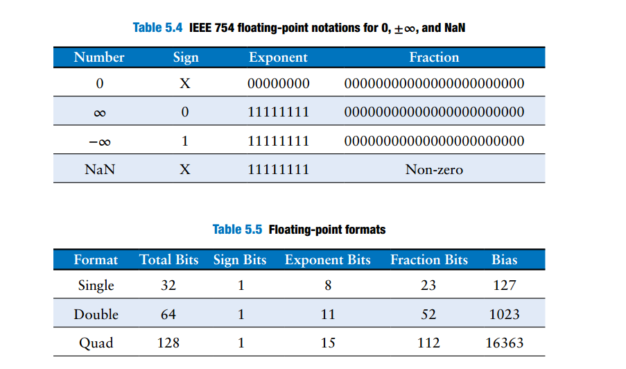
Floating-point Number in IEEE 754 Format

Floating-point data in IEEE 754 Format [https://github.com/IC-Design-Lab/IC-Design/blob/main/Training/Floating-point%20data%20in%20IEEE%20754%20Format.pdf]

Rajaraman, V.. “IEEE standard for floating point numbers.” Resonance 21 (2016): 11 - 30. [https://www.ias.ac.in/article/fulltext/reso/021/01/0011-0030]

IEEE Standard for Floating-Point Arithmetic [https://www-users.cse.umn.edu/~vinals/tspot_files/phys4041/2020/IEEE%20Standard%20754-2019.pdf]

Dennis Forbes. Understanding Floating-Point Numbers [https://dennisforbes.ca/blog/features/floating_point/understanding-floating-point-numbers/]

Bevan Baas, EEC 281 - VLSI Digital Signal Processing Winter 2025 [FLOATING POINT] [FLOATING POINT <---> FIXED POINT CONVERSION]

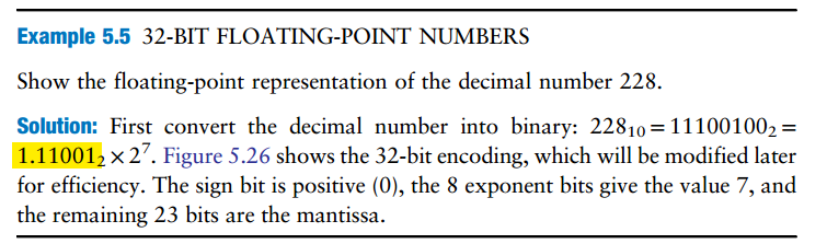
32-bit floating-point version 1	store implicit leading one
32-bit floating-point version 2	discard implicit leading one
IEEE 754 floating point notation	*biased exponent*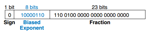

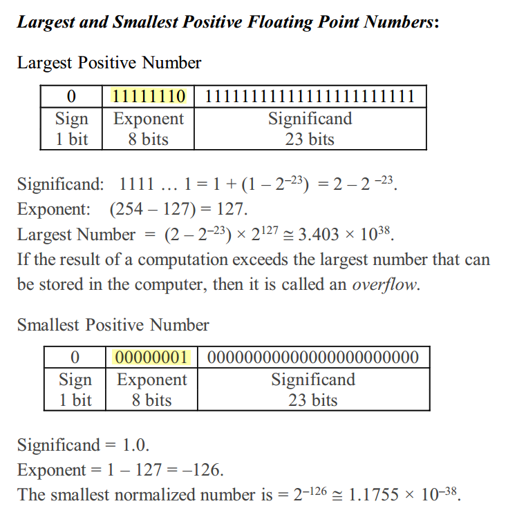\[ \boxed{ \begin{aligned} E=0 &: \quad \text{zero or subnormal},\\ 1\le E\le254 &: \quad \text{normal finite number},\\ E=255 &: \quad \infty \text{ or NaN}. \end{aligned} } \]

2's Complement

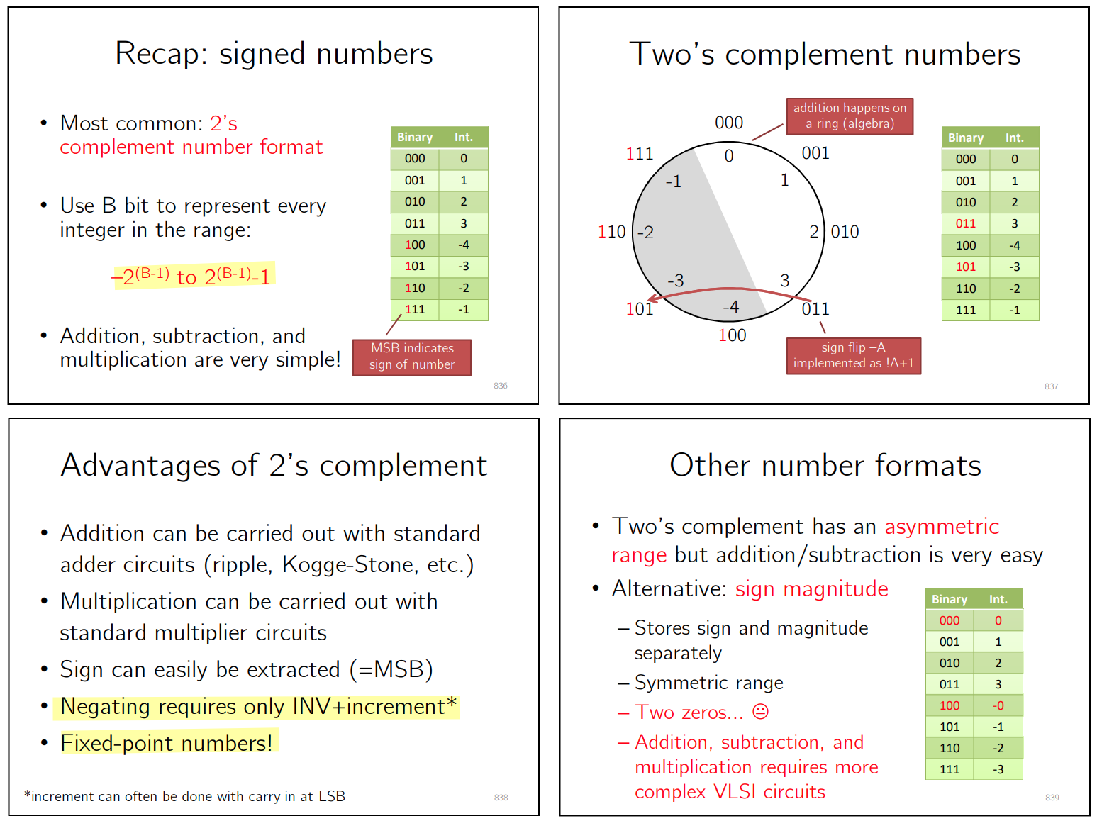
[https://bpb-us-w2.wpmucdn.com/sites.coecis.cornell.edu/dist/4/81/files/2019/06/4740_lecture23ALU-circuits.pdf]

2's complement negative number

Flip all bits then Add 1

N-bit signed number \[ A = -M_{N-1}2^{N-1}+\sum_{k=0}^{N-2}M_k2^k \] Flip all bits \[\begin{align} A_{flip} &= -(1-M_{N-1})2^{N-1} +\sum_{k=0}^{N-2}(1-M_k)2^k \\ &= M_{N-1}2^{N-1}-\sum_{k=0}^{N-2}M_k2^k -2^{N-1}+\sum_{k=0}^{N-2}2^k \\ &= M_{N-1}2^{N-1}-\sum_{k=0}^{N-2}M_k2^k -1 \end{align}\]

Add 1 \[ A_- = A_{flip}+1 = M_{N-1}2^{N-1}-\sum_{k=0}^{N-2}M_k2^k = -A \]

negative number to 2's complement, interpreted as unsigned number \[ \text{S} = -2^{N-1} + \text{LSBs} \qquad \Longrightarrow \qquad \text{S} + 2^N = 2^{N-1} + \text{LSBs} \] For example -2 in 3-bit 2's complement is -2 + 8 = 6 = 3'110

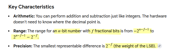
Fixed Point Number

Different notations can be used to represent different fractional formats

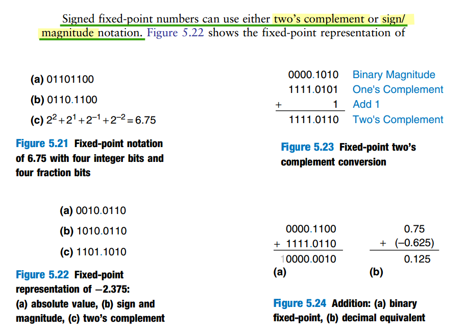
Q format; Wordlength, Fractionlength Format

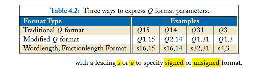
Different sources use slightly different $Q$-format conventions

$Q1.3$ means that the 1 includes the sign bit. \[ Q1.3 = \underbrace{1\text{ bit}}_{\text{sign / integer side}} + \underbrace{3\text{ fractional bits}}_{\text{fractional side}} \] So it is a 4-bit two's-complement fixed-point number:

1
2
3

 b3 . b2 b1 b0
 ↑      ↑ ↑ ↑
sign    3 fractional bits

Bit Shifts: Gain Scaling & Format Conversion

multiplication or format conversion

For a fixed-point number, distinguish the stored integer $X$ from the represented value $x$:

\[ \color{blue}\boxed{x=\frac{1}{2^F}X} \]

Here, $F$ is the number of fractional bits. The binary point is an interpretation of the bits; it is not physically stored

1	assign ted_s5_3 = (ted_s2_0 << 3); //s2.0 -> S5.3

The stored integer is multiplied by 8, while the fractional-bit count increases from zero to 3:

\[ Y=2^3 X,\qquad y=Y\,2^{-3}=X=x \]

For an input value of +1:

Interpretation	Stored bits	Fractional bits	Represented value
Original `S2.0`	`01`	0	1
Shifted result interpreted as `S5.0`	`01000`	0	8	multiplication
Shifted result interpreted as `S5.3`	`01000`	3	1	format conversion

Thus, the same shift can implement multiplication or a format conversion, depending on the output scale.

SystemVerilog performs the bit operation
your format convention determines its numerical meaning

module Ar_B (
    input  [12:0] A,  // ratio
    input  [11:0] B,  // offset
    input  [11:0] r,  // raw output
    output [12:0] So  // post-processed output
);

// So(r) = g(r) = A*(r/2^12) - B
//
// r: 12-bit unsigned integer.
//
// A: 13 bits.
//    bit[12:4] integer.
//    bit[3:0]  fractional.
//
// B: 12 bits.
//    bit[11:4] integer.
//    bit[3:0]  fractional.
//
// So: 13 bits.
//     bit[12]   sign bit.
//     bit[11:4] integer.
//     bit[3:0]  fractional.

wire [25:0] So_tmp;
wire [25:0] A_tmp;
wire [25:0] B_tmp;
wire [25:0] So_int;
wire        sign_tag;

assign B_tmp    = (B[11:0] << 12);
assign A_tmp    = A[12:0] * r[11:0];
assign So_tmp   = (A_tmp > B_tmp) ? (A_tmp - B_tmp)
                                      : (B_tmp - A_tmp);
assign sign_tag = (B_tmp > A_tmp);
assign So_int   = (So_tmp >> 12);

assign So[12:0] = {sign_tag, So_int[11:0]};  // sign-magnitude encoding

endmodule

Let the unsigned stored codes be $A$, $B$, and $r$. The intended values are:

\[ a=\frac{A}{2^4},\qquad b=\frac{B}{2^4} \]

so the desired output is:

\[ g=a\frac{r}{2^{12}}-b =\boxed{\frac{Ar-B\,2^{12}}{2^{16}}} \]

Consequently, the intermediate signals can be interpreted as follows:

Signal	Stored integer	Fractional bits	Represented value
`A_tmp`	$Ar$	16	$a(r/2^{12})$
`B_tmp`	$B\,2^{12}$	16	$b$
`So_tmp`	$\lvert Ar-B\,2^{12}\rvert$	16	$\lvert g\rvert$
`So_int`	$\left\lfloor\texttt{So}_\texttt{tmp}/2^{12}\right\rfloor$	4	$\lvert g\rvert$ quantized downward to steps of $1/16$

Here, B << 12 converts the offset from 4 fractional bits to 16, preserving its represented value. Likewise, So_tmp >> 12 converts the magnitude from 16 fractional bits to 4, discarding precision.

Let $A$ denote the stored integer code. Since $A$ has four fractional bits:

\[ a=\frac{A}{2^4} \]

The multiplication produces the stored integer:

\[ P=Ar \]

Its interpretation depends on the quantity we want it to represent:

Intended quantity	Relationship to stored product $P$	Fractional bits
$a\,r$	$a\,r=P/2^4$	4
$a(r/2^{12})$	$a(r/2^{12})=P/2^{16}$	16

The extra 12 fractional bits come from including the normalization by $2^{12}$ in the interpretation. The multiplication itself does not add them automatically

Both interpretations are valid. For your complete calculation, the second makes the alignment particularly clear:

\[ g=\frac{\underbrace{Ar}_{\text{16 fractional bits}} -\underbrace{B\,2^{12}}_{\text{16 fractional bits}}}{2^{16}} \]

Here, both numerator terms are stored codes using the same scale, $2^{-16}$

right shift effect

1	assign So_int = (So_tmp >> 12);

$rshift_frac.drawio$

Signal	Stored integer	Fractional bits	Represented value
`So_int`	$\left\lfloor\texttt{So}_\texttt{tmp}/2^{12}\right\rfloor$	4	$\lvert g\rvert$ quantized downward to steps of $1/16$

left shift effect

logic signed [5:0] obj_s6_3;		// S6.3
logic signed [15:0] prop_s16_16;	// S16.16

prop_s16_16 = obj_s6_3 << 10;	// gain = 1/2^3

The gain from obj_s6_3 to prop_s16_16 \[ \left\{ \begin{array}{cl} x&=\frac{X}{2^3} \\ y&=X 2^{10}\cdot \frac{1}{2^{16}}=\frac{X}{2^6}\end{array} \right. \qquad \Longrightarrow \qquad y=\frac{1}{2^3}\cdot x \] Generally, a left shift by $k$ with input/output fractional-bit counts $F_{\text{in}}$ and $F_{\text{out}}$ gives:

\[ \boxed{y=2^{k+F_{\text{in}}-F_{\text{out}}}x} \]

provided no bits are lost

Programmable gain scaling

module fixed_point_gain (
    input  logic signed [5:0]  data_in,  // S6.2
    input  logic        [1:0]  gain_sel,
    output logic signed [23:0] data_out  // S24.19
);

    logic signed [15:0] gain_scaled;     // S16.11

    always_comb begin
        case (gain_sel)
            2'd0:    gain_scaled = data_in << 10; // Gain = 2
            2'd1:    gain_scaled = data_in << 9;  // Gain = 1
            2'd2:    gain_scaled = data_in << 8;  // Gain = 1/2
            2'd3:    gain_scaled = data_in << 7;  // Gain = 1/4
            default: gain_scaled = '0;
        endcase
    end

    // S16.11 -> S24.19: preserve the represented value.
    assign data_out = gain_scaled << 8;

endmodule

Let $X$ be the signed input code and $k$ the first-stage shift:

\[ x=X2^{-2}, \qquad y=(X2^k2^8)2^{-19} =\boxed{x\,2^{k-9}} \]

`gain_sel`	Shift (k)	Numerical gain
`0`	10	2
`1`	9	1
`2`	8	1/2
`3`	7	1/4

The widths are sufficient

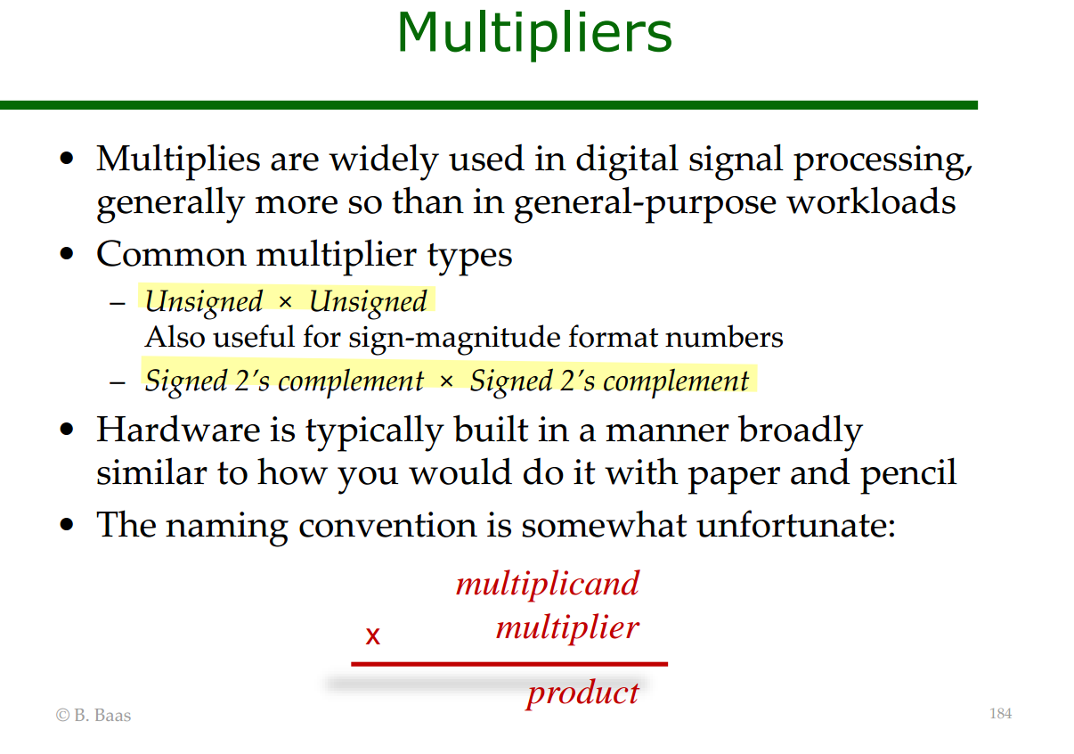
Multiplication

B. Baas, [HARDWARE MULTIPLIERS] [FIXED-INPUT MULTS] [MULTIPLICATION SCALING]

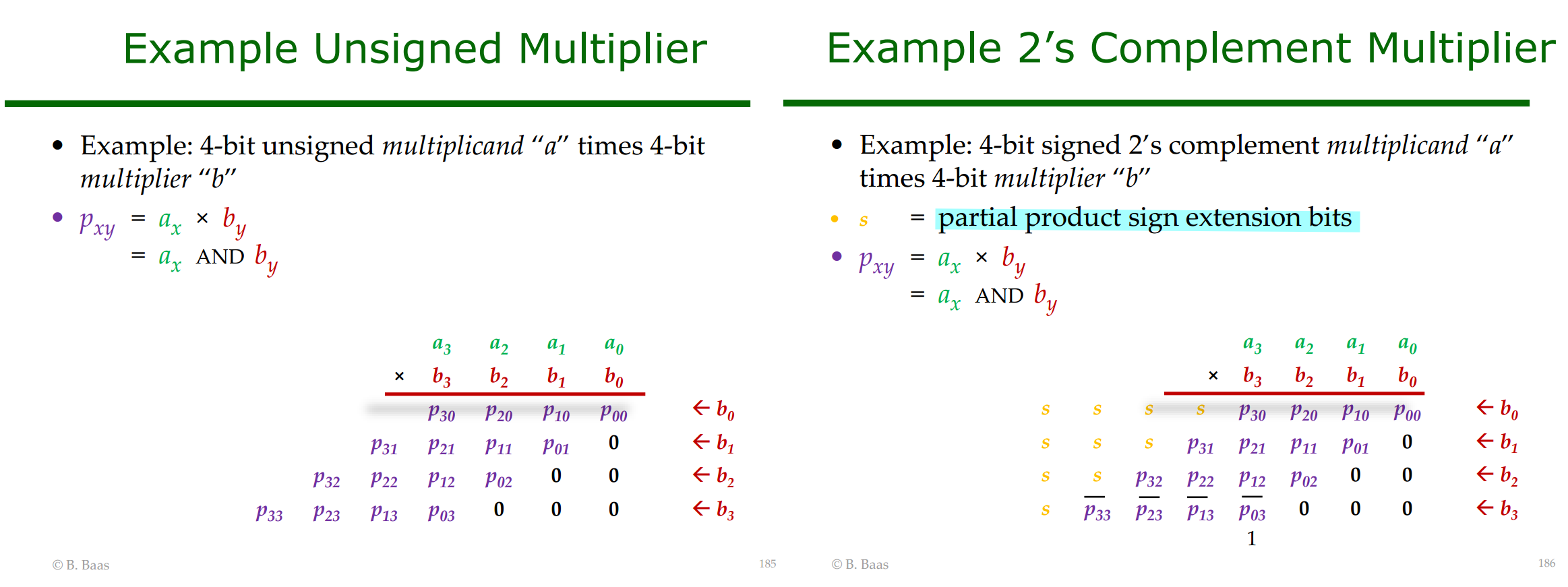
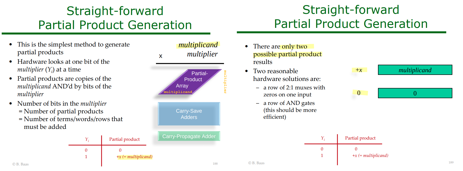
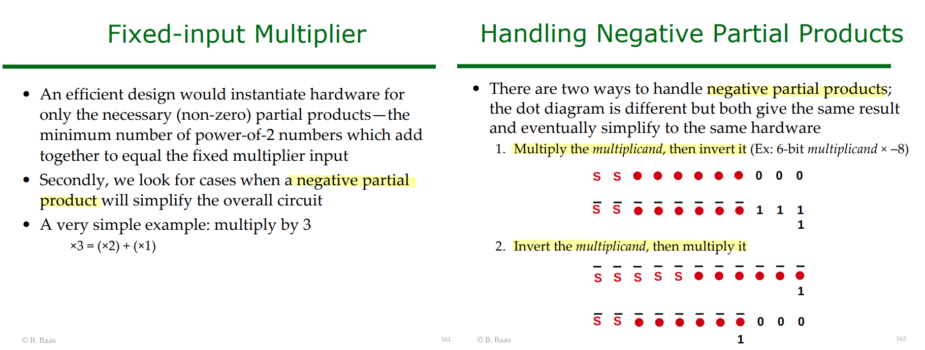
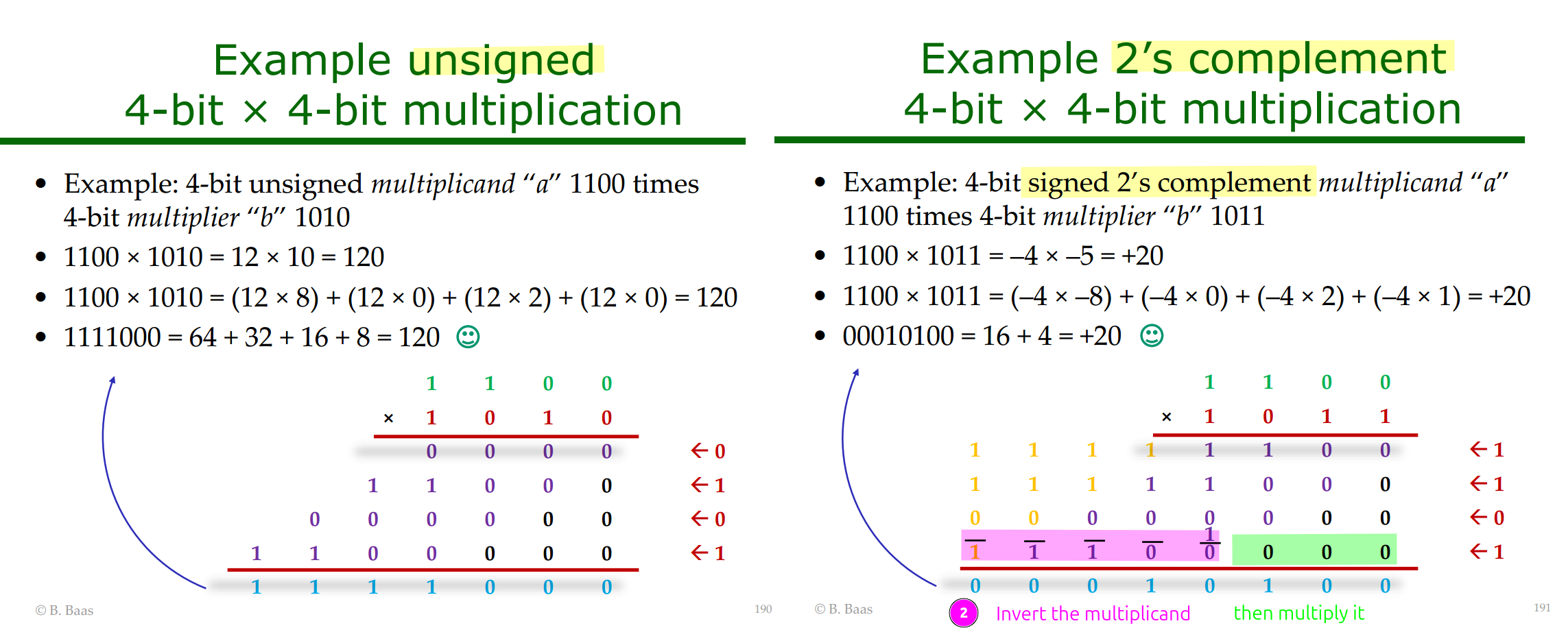
negate last partial product when multiplier[MSB]=1, i.e. multiplier is negative

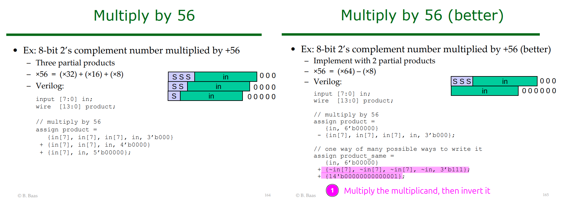
Multiply the multiplicand, then invert it
Invert the multiplicand, then multiply it

Multiplication Scaling

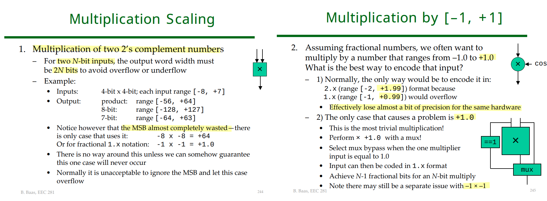
product wordlength

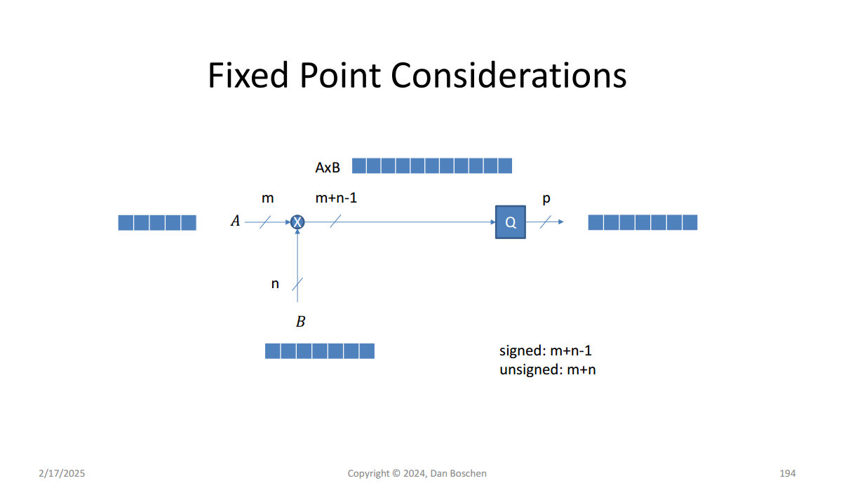
Operands	Nominal full product width
Unsigned	$m+n$	no overflow for any case
Signed fractional	$m+n-1$	with the exception of `(-1)*(-1)` case

For signed fractional multiplication,

\[ Q1.(m-1)\times Q1.(n-1) \rightarrow Q1.(m+n-2) \]

Therefore, the total number of bits is

\[ 1+(m+n-2)=m+n-1. \]

There is one special corner case:

\[ (-1)\times(-1)=+1 \]

but a signed fractional format such as $Q1.(m+n-2)$ has the range

\[ -1 \le x \le 1-2^{-(m+n-2)}, \]

so it cannot represent exactly $+1$.

Therefore:

Normally, signed fractional multiplication requires

\[ \boxed{m+n-1\text{ bits}} \]

To guarantee no overflow even for

\[ (-1)(-1)=+1, \]

you need

\[ \boxed{m+n\text{ bits}} \]

Equivalently, if the operands have widths

\[ B_0+1 \quad\text{and}\quad B_1+1, \]

then the normal signed fractional product width is

\[ (B_0+1)+(B_1+1)-1 = \boxed{B_0+B_1+1}. \]

The only exception is again

\[ (-1)(-1)=+1 \]

Alan V Oppenheim, Ronald W. Schafer. Discrete-Time Signal Processing, 3rd edition

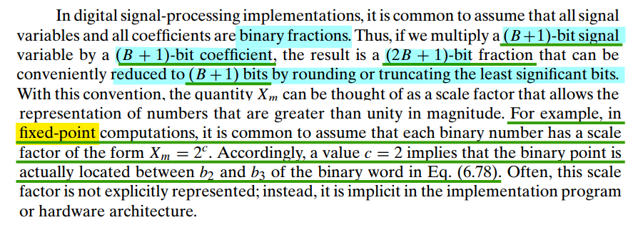
The useful fixed-point multiplication rule is \[ Q_{F_1} \times Q_{F_2} \qquad \Longrightarrow\qquad F_{\text{product}} = F_1 + F_2 \] where $F_1$ and $F_2$ are the numbers of fractional bits of the two operands

4-bit words are

1 2	a = 0.100 -> 0100 y_hat = 0.111 -> 0111

Now temporarily ignore the binary point and multiply the integer bit patterns:

   0100        (= 4)
 × 0111        (= 7)
 -------
   0100
  0100
 0100
0000
 -------
0011100        (= 28)

Multiplying an $M$-bit signed number by an $N$-bit signed number requires at most $M+N$ signed bits to avoid overflow, assuming two’s-complement representation and that $M,N$ include the sign bits.

The corner case is the most negative value multiplied by the most negative value:

\[ (-2^{M-1})(-2^{N-1})=+2^{M+N-2} \]

An $(M+N-1)$-bit signed result can only represent positive values up to

\[ 2^{M+N-2}-1 \]

so it is one count short. Hence $M+N$ bits are necessary for the full input range.

For example, two signed 3-bit numbers can each equal $-4$:

\[ (-4)(-4)=16 \]

Signed 5-bit range: $[-16,15]$ → overflow.
Signed 6-bit range: $[-32,31]$ → fits.

For fixed-point multiplication, the fractional lengths also add:

\[ \boxed{W_{\text{out}}=M+N,\qquad F_{\text{out}}=F_a+F_b} \]

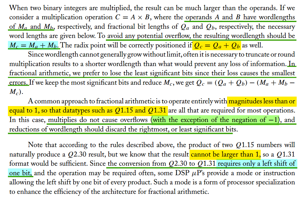
For the conversion $Q2.30\rightarrow Q1.31$, both formats have 32 total bits:

Format	Stored integer	Represented value
$Q2.30$	$P$	$P\,2^{-30}$
$Q1.31$ after shifting left	$2P$	$(2P)\,2^{-31}$

Therefore, provided no overflow occurs,

\[ \boxed{x_{\text{after}}=(2P)\,2^{-31}=P\,2^{-30}=x_{\text{before}}} \]

For a 32-bit left shift converting $Q2.30\rightarrow Q1.31$, overflow is avoided only when the original two MSBs are identical:

Original two MSBs	Original $Q2.30$ value $x$	Conversion
`00`	$0\le x<1$	Safe
`11`	$-1\le x<0$	Safe
`01`	$1\le x<2$	Positive overflow
`10`	$-2\le x<-1$	Negative overflow

The shift discards the original MSB, and the second MSB becomes the new sign bit. When they match, the discarded bit is a redundant sign-extension bit, so the value is preserved after adjusting the fractional length

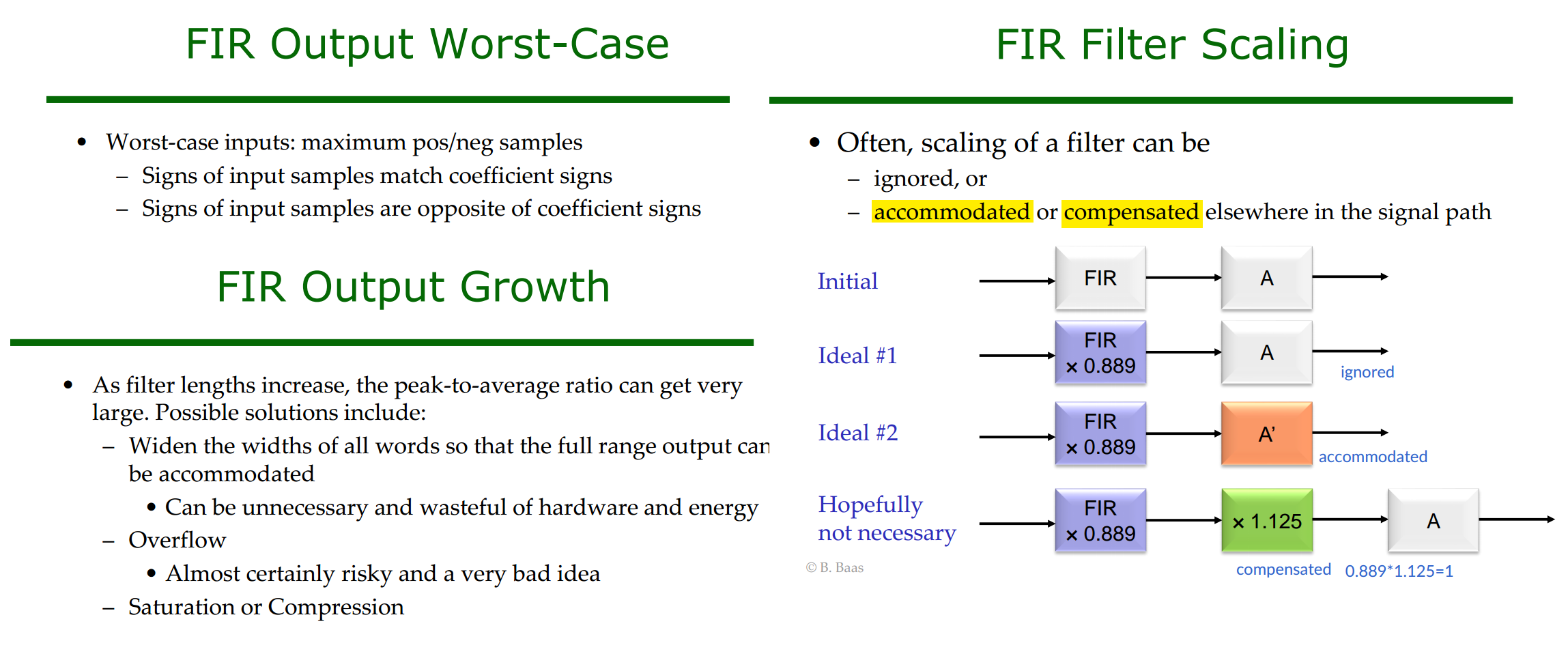
FIR Filter Scaling

Bevan Baas, EEC 281 - VLSI Digital Signal Processing Winter 2025 [FIR FILTER HARDWARE]

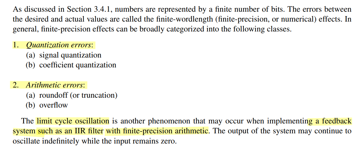
Finite-wordlength Effects

Tianshuang Qiu; Ying Guo, "7. Finite-Precision Numerical Effects in Digital Signal Processing," in Signal Processing and Data Analysis , De Gruyter, 2018, pp.236-248

Antoniou, Andreas. “Digital Signal Processing: Signals, Systems, and Filters.” (2005). [pdf]

Alan V Oppenheim, Ronald W. Schafer. Discrete-Time Signal Processing, 3rd edition

Bevan Baas, EEC 281 - VLSI Digital Signal Processing Winter 2025 [QUANTIZATION NOISE AS A FUNCTION OF WORD SIZE] [SATURATION&COMPRESSION] [ROUNDING]

Keshab K. Parhi, Chapter 11: Scaling and Round-off Noise [http://www.ece.umn.edu/users/parhi/SLIDES/chap11.pdf]

image-2026-08-11_12-38

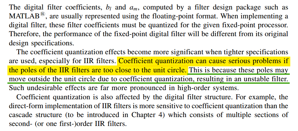
Coefficient Quantization

Roundoff Noise

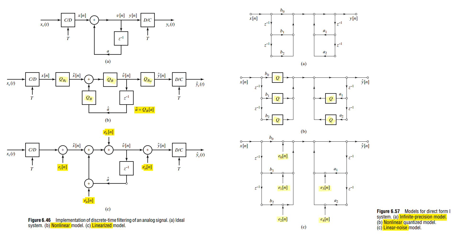
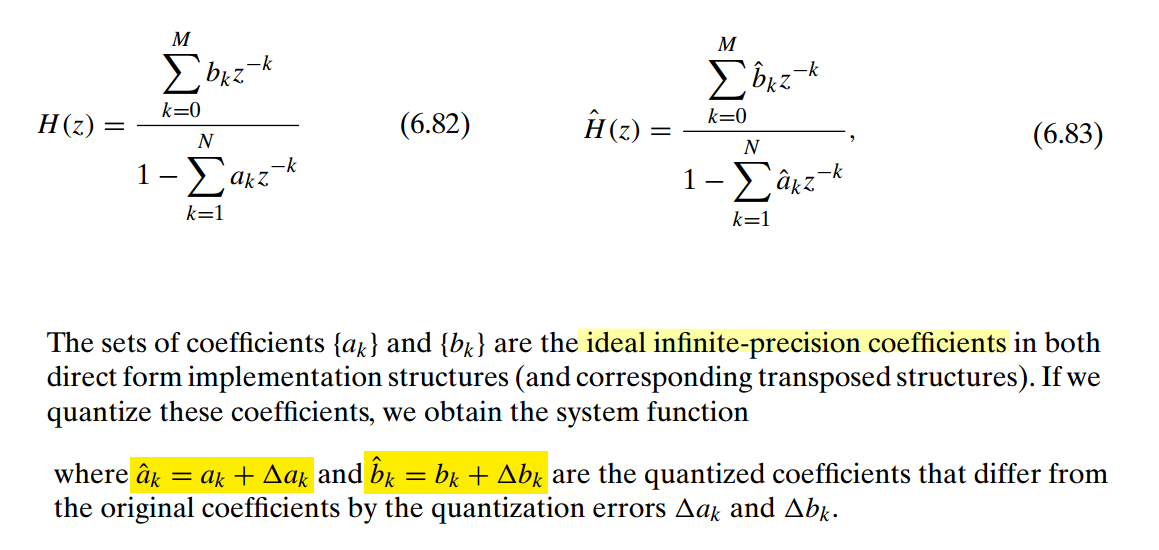
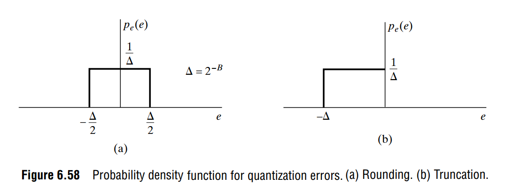
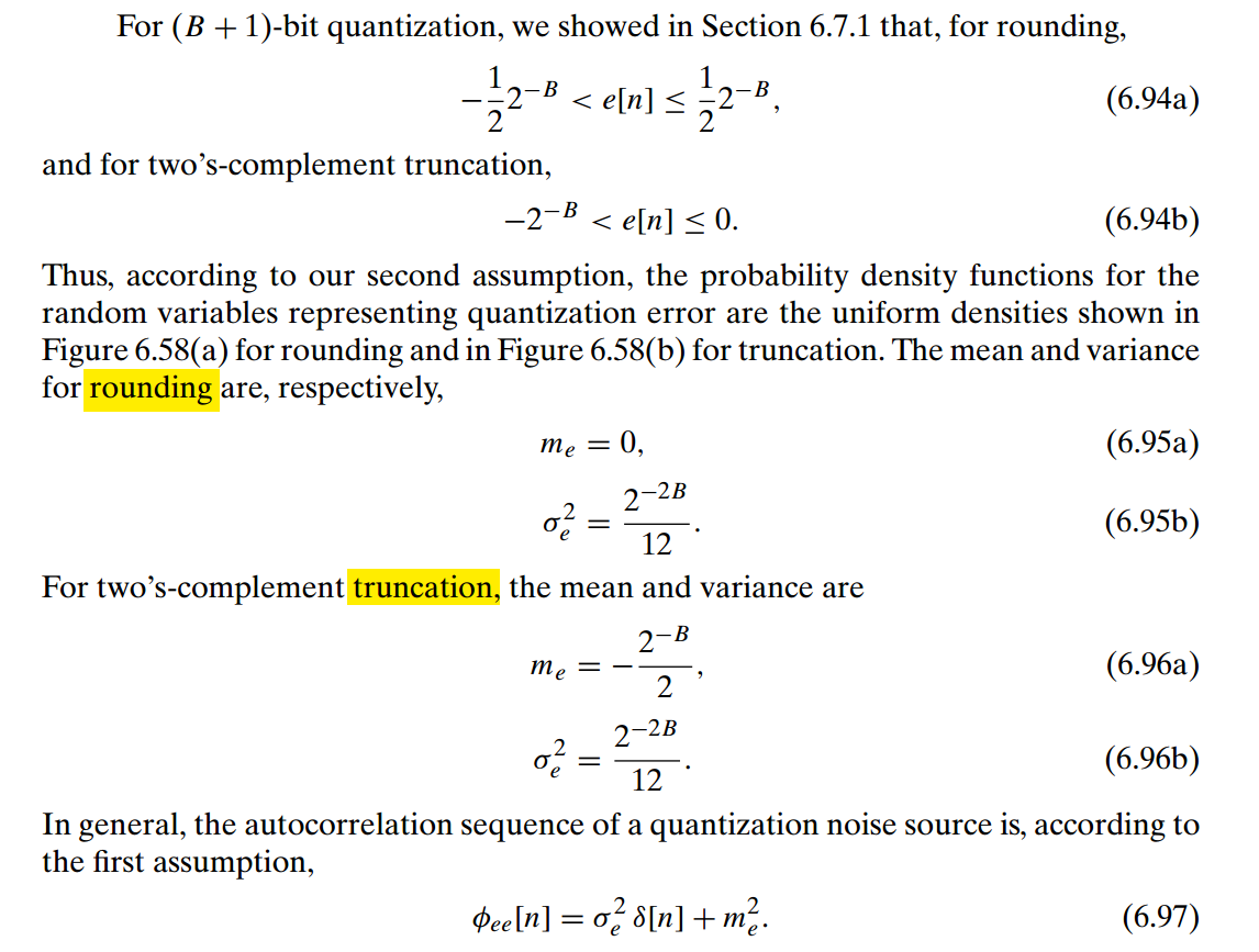
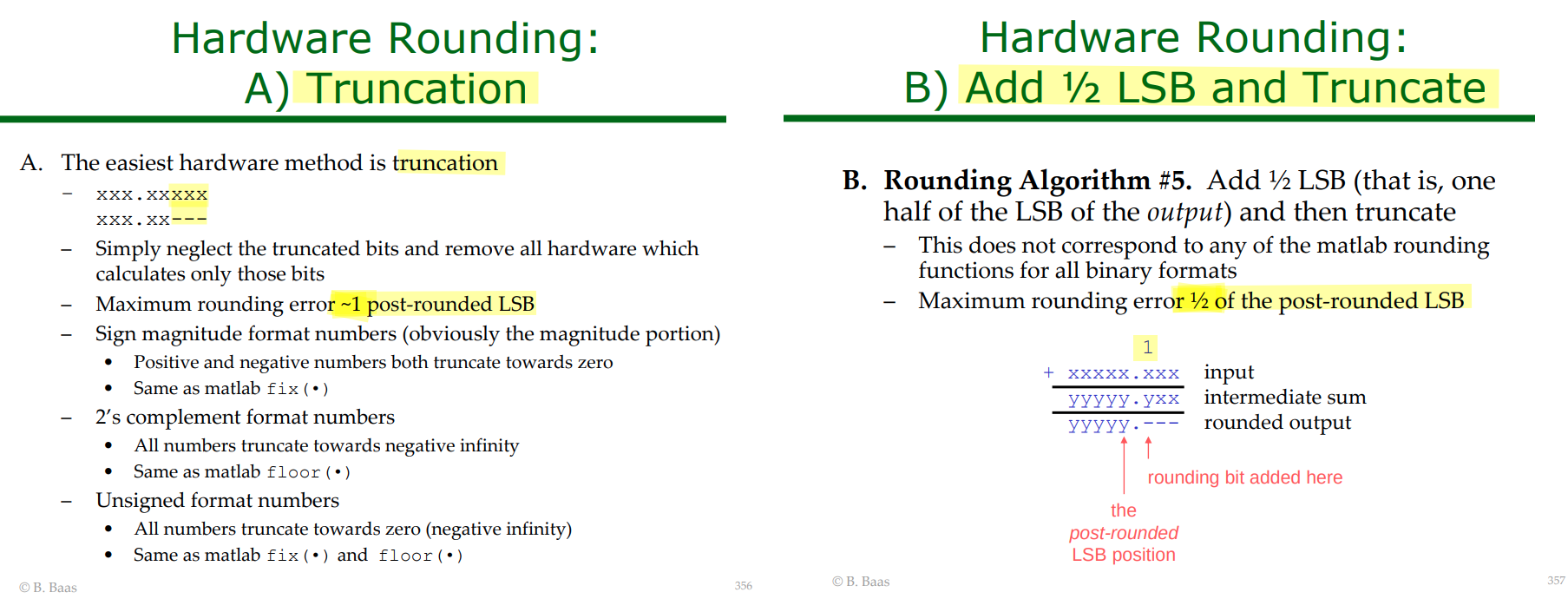
Direct-Form I (DF-I) implementation of a digital filter IIR

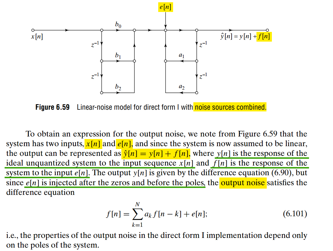
Equation (6.101) follows directly by writing the difference equation for the quantized system and subtracting the difference equation for the ideal system.

For the direct-form-I filter in Fig. 6.59, the ideal output satisfies

\[ y[n] = \sum_{k=0}^{M} b_k x[n-k] + \sum_{k=1}^{N} a_k y[n-k]. \tag{1} \]

The combined quantization noise $e[n]$ is injected after the $b_k$ section (zeros) and before the $a_k$ feedback section (poles). Therefore the actual output $\hat y[n]$ satisfies

\[ \hat y[n] = \sum_{k=0}^{M} b_k x[n-k] + \sum_{k=1}^{N} a_k \hat y[n-k] + e[n]. \tag{2} \]

The book defines

\[ \boxed{\hat y[n]=y[n]+f[n]} \]

where $f[n]$ is the output component caused by the quantization noise

Substitute

\[ \hat y[n]=y[n]+f[n] \]

into (2):

\[ y[n]+f[n] = \sum_{k=0}^{M}b_kx[n-k] + \sum_{k=1}^{N}a_k\left(y[n-k]+f[n-k]\right) + e[n]. \]

Expand:

\[ y[n]+f[n] = \underbrace{ \sum_{k=0}^{M}b_kx[n-k] + \sum_{k=1}^{N}a_ky[n-k] }_{=\,y[n]} + \sum_{k=1}^{N}a_kf[n-k] + e[n]. \]

Using the ideal-system equation (1),

\[ y[n]+f[n] = y[n] + \sum_{k=1}^{N}a_kf[n-k] + e[n]. \]

Cancel $y[n]$ from both sides:

\[ \boxed{ f[n] = \sum_{k=1}^{N}a_k f[n-k]+e[n] } \tag{6.101} \]

That is exactly Eq. (6.101).

Why do the $b_k$ coefficients disappear?

This is the important point.

The signal path is

\[ x[n] \rightarrow \underbrace{B(z)}_{\text{zeros}} \rightarrow \boxed{+\,e[n]} \rightarrow \underbrace{\frac{1}{A(z)}}_{\text{poles}} \rightarrow \hat y[n]. \]

The noise is inserted after $B(z)$, so it never passes through the zeros. It only passes through the all-pole feedback section.

In the $z$-domain, Eq. (6.101) gives

\[ F(z) = \sum_{k=1}^{N}a_kz^{-k}F(z)+E(z). \]

Thus,

\[ F(z) \left( 1-\sum_{k=1}^{N}a_kz^{-k} \right) = E(z), \]

and therefore

\[ \boxed{ \frac{F(z)}{E(z)} = \frac{1} {1-\displaystyle\sum_{k=1}^{N}a_kz^{-k}} } \]

So the output quantization-noise transfer function contains only the poles, which is what the sentence immediately after (6.101) means.

For the second-order example in the figure,

\[ \boxed{ f[n]=a_1f[n-1]+a_2f[n-2]+e[n]. } \]

The coefficients $b_0,b_1,b_2$ have no effect on $f[n]$ because $e[n]$ is injected after that part of the filter.

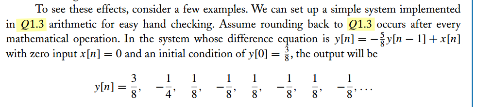
Limit Cycles in feedback system

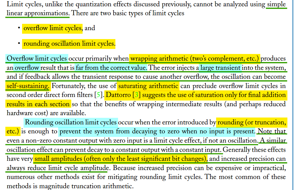
Limit Cycles Owing to Round-off & Truncation

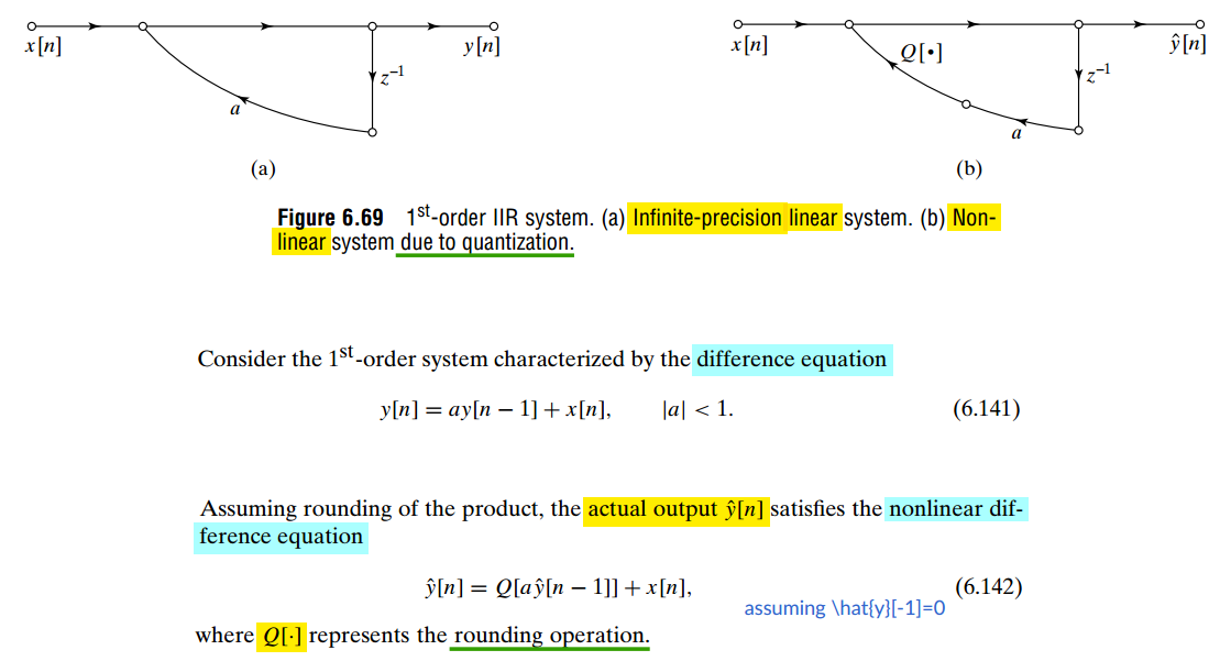
For infinite-precision linear system $y[n] = a y[n-1] + x[n],$

with zero initial condition $y[-1]=0$, the impulse response is \[ y[n] = \frac{7}{8} a^n u[n] \] because after the impulse at $n=0$, we have $x[n]=0$ for all $n\ge 1$.

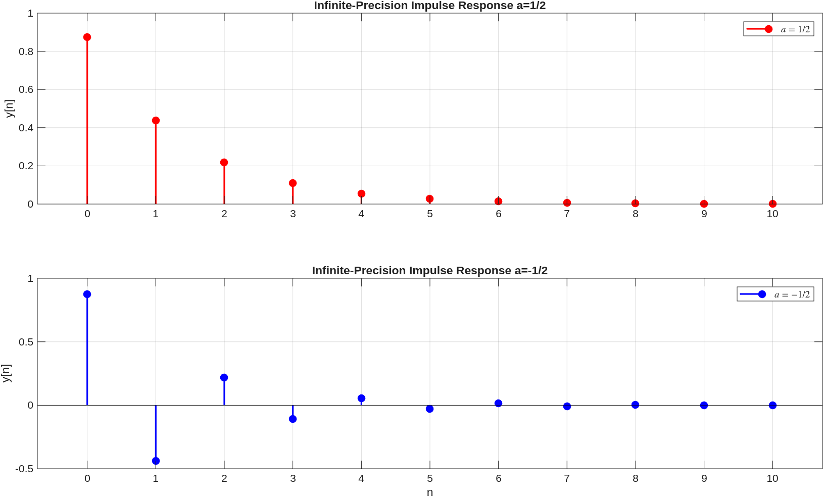
For nonlinear system $\hat{y}[n] = Q[a \hat{y}[n-1]] + x[n],$

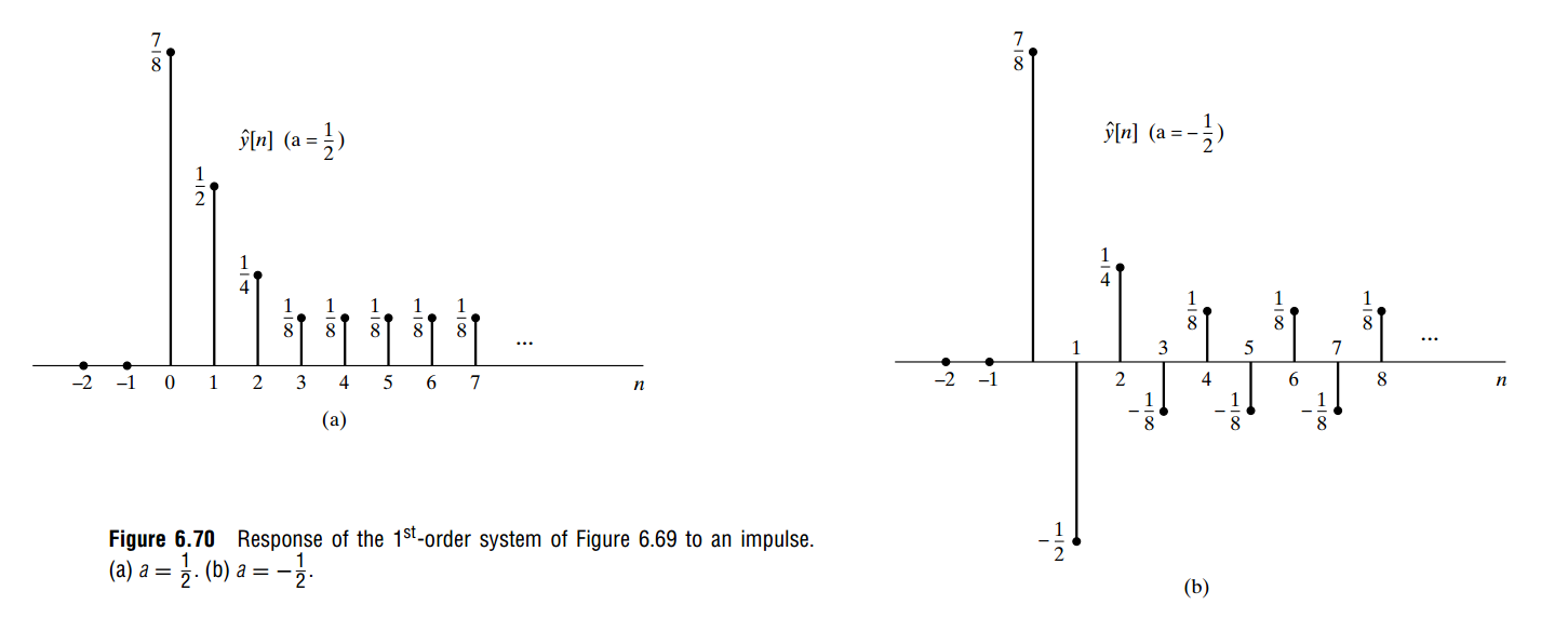
The nonzero steady oscillation or constant value is created entirely by the rounding operation (nonlinear) $Q[\cdot]$

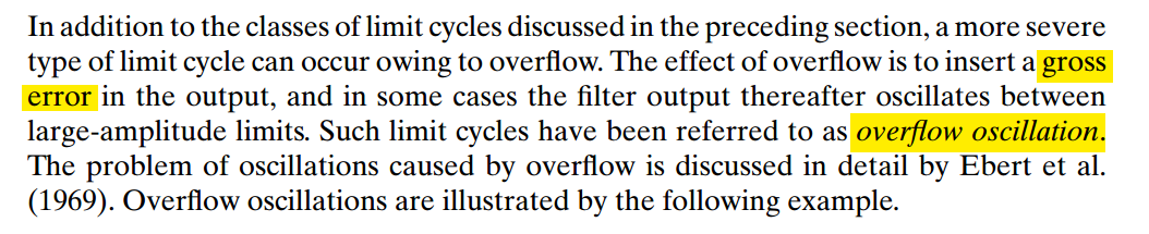
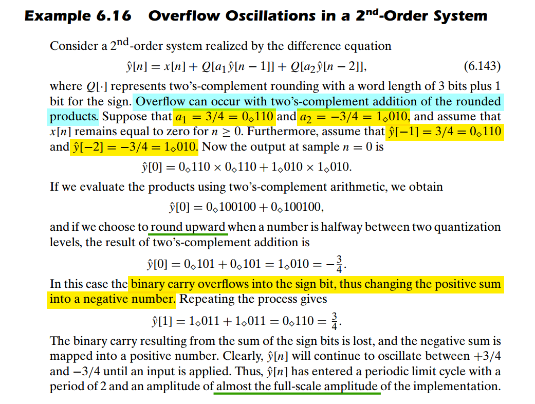
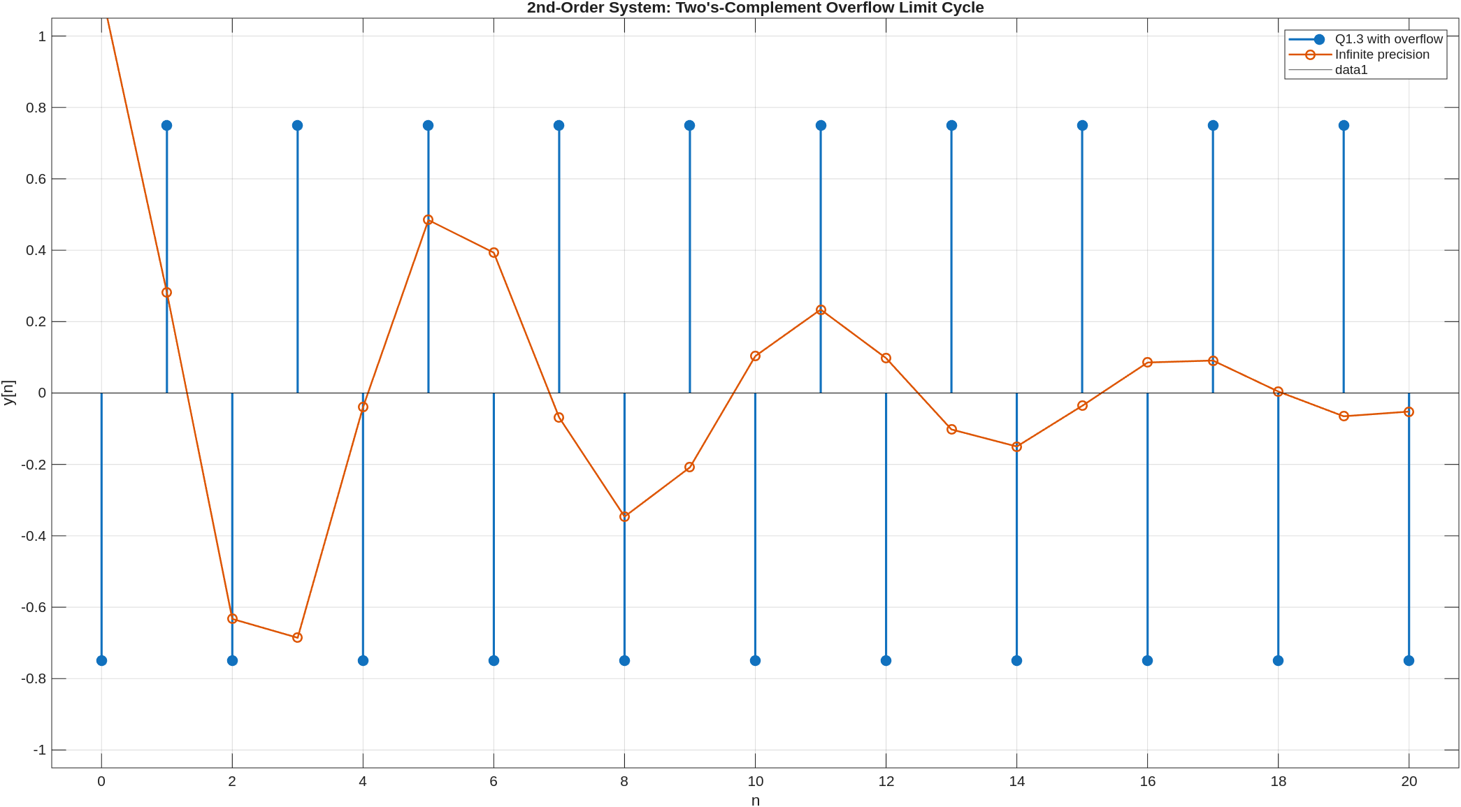
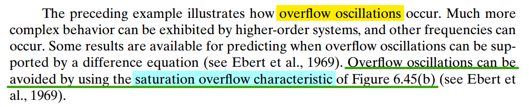
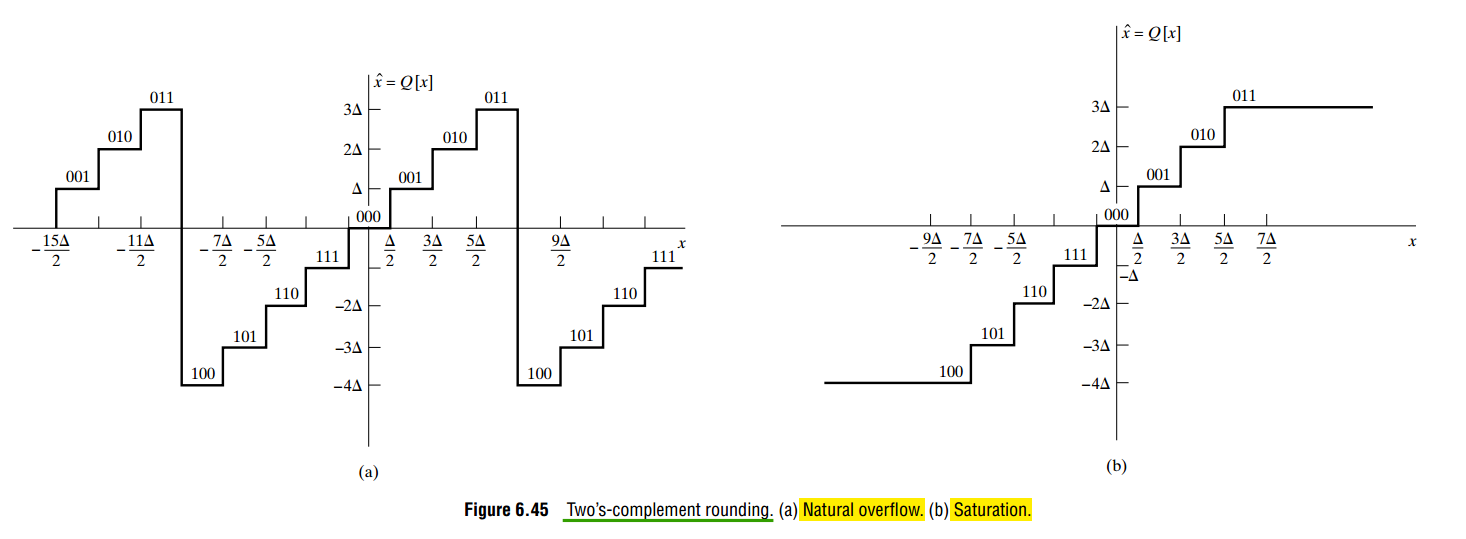
Limit Cycles Owing to Overflow

%% Parameters
a1 =  3/4;
a2 = -3/4;

% Q1.3:
% 1 sign/integer bit + 3 fractional bits
F  = 3;               % fractional bits
WL = 4;               % total word length
S  = 2^F;             % scale factor = 8

% Initial conditions
% y[-2] = -3/4
% y[-1] = +3/4
y_m2 = -3/4;
y_m1 =  3/4;

N = 20;
n = 0:N;


%% ------------------------------------------------------------
%  Finite-precision Q1.3 system
% -------------------------------------------------------------

yq = zeros(size(n));

% Store the two previous states
ym2 = y_m2;
ym1 = y_m1;

for k = 1:length(n)

    % Products
    p1 = a1 * ym1;
    p2 = a2 * ym2;

    % Round products back to Q1.3.
    % Halfway cases are rounded away from zero:
    %
    %   +9/16 -> +5/8
    %   -9/16 -> -5/8
    %
    p1q = sign(p1) * floor(abs(p1)*S + 0.5) / S;
    p2q = sign(p2) * floor(abs(p2)*S + 0.5) / S;

    % Addition
    s = p1q + p2q;

    % Two's-complement overflow / wraparound
    %
    % Convert to integer representation first
    sint = round(s*S);

    % Wrap to WL-bit signed two's-complement range
    sint = mod(sint + 2^(WL-1), 2^WL) - 2^(WL-1);

    % Convert back to Q1.3
    yq(k) = sint / S;

    % Update states
    ym2 = ym1;
    ym1 = yq(k);
end


%% ------------------------------------------------------------
%  Infinite-precision system
% -------------------------------------------------------------

yinf = zeros(size(n));

ym2 = y_m2;
ym1 = y_m1;

for k = 1:length(n)

    yinf(k) = a1*ym1 + a2*ym2;

    ym2 = ym1;
    ym1 = yinf(k);
end

//-------------------------------------------------------------------------
// Recombine and saturate: dac = clamp(x_msb + y, 0, 2^OUT_W-1)
//   sum range [-3, 2^OUT_W-1+4] -> (OUT_W+2)-bit signed is sufficient
//   (needs 2^(OUT_W+1) >= 2^OUT_W + 4, true for any OUT_W >= 2)
//-------------------------------------------------------------------------
// explicit sign-extension of y to adder width (assumes OUT_W >= 5)
wire signed [OUT_W+1:0] y_ext   = {{(OUT_W-4){y[5]}}, y};
wire signed [OUT_W+1:0] dac_sum = $signed({2'b0, x_msb}) + y_ext;

wire [OUT_W-1:0] dac_sat =
      dac_sum[OUT_W+1] ? {OUT_W{1'b0}} :   // negative  -> 0
      dac_sum[OUT_W]   ? {OUT_W{1'b1}} :   // > max     -> 2^OUT_W-1
      dac_sum[OUT_W-1:0];

Avoiding Limit Cycles

The suppression of limit cycles is a broad topic with all the complexity to be expected in a nonlinear system behavior.

The most basic tools of saturation arithmetic and magnitude truncation — rounding rounds toward zero

Saturation Arithmetic & Scaling of Signals

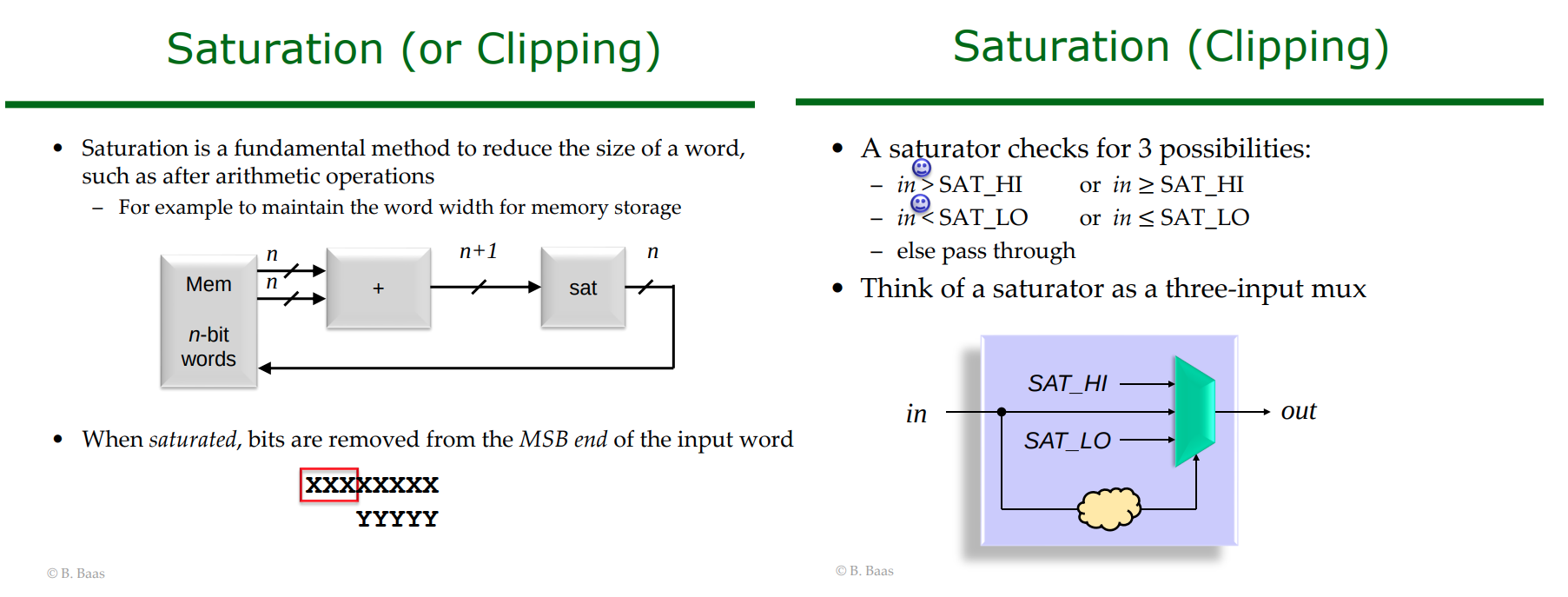
Saturation arithmetic prevents overflow by clipping the results to a maximum value

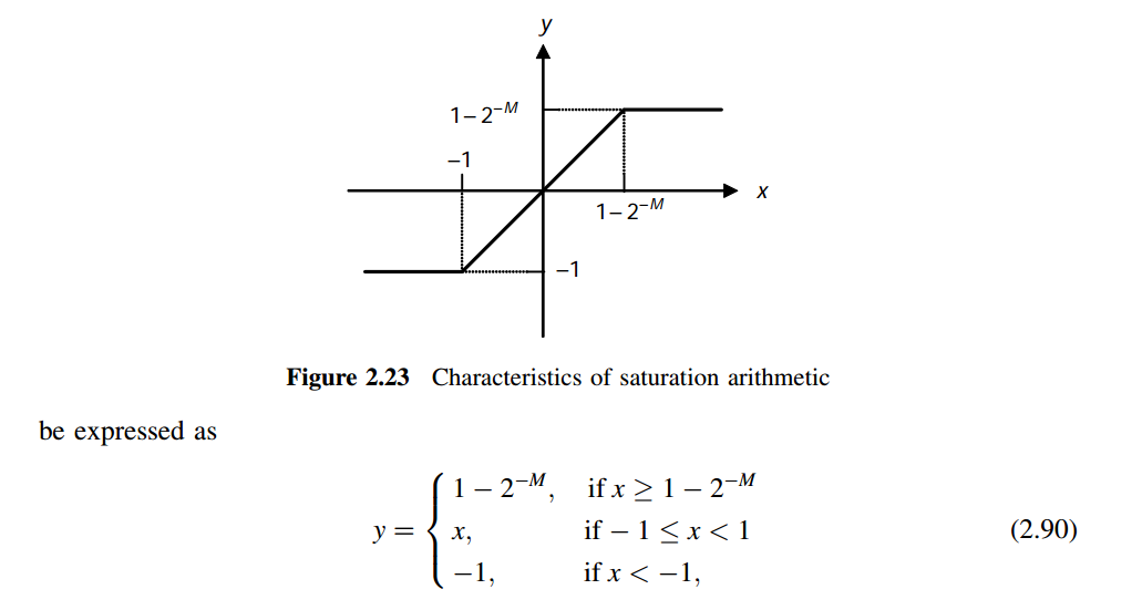
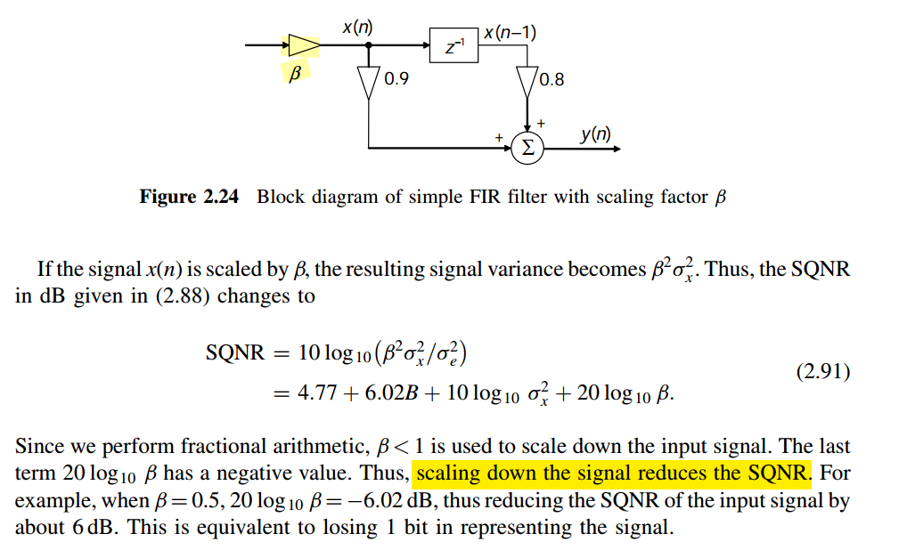
The most effective technique in preventing overflow is by scaling down the signal

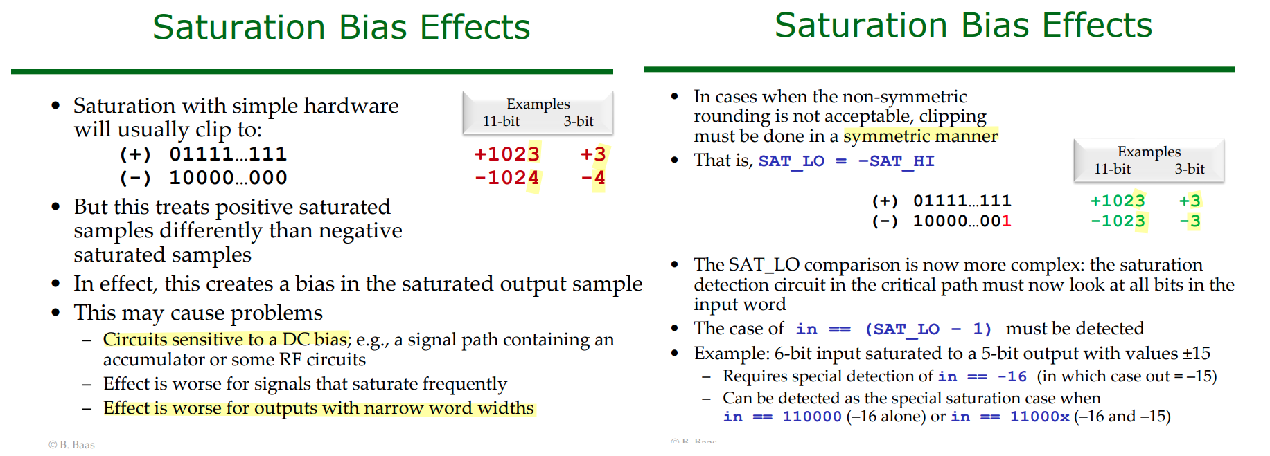
Saturation Bias Effects

One-Hot and Thermometer (Unary) codes

An N-bit binary input represents $2^{N}$ unique values (from 0 to $2^N - 1$)

Converting this input requires a $2^{N}$-bit width for One-Hot encoding, but only a $(2^N - 1)$-bit width for Thermometer Code, as the value zero is represented by all zeros

Decimal	Binary ($N=3$)	One-Hot ($2^3 = 8$) bits)	Thermometer ($2^3 - 1 = 7$) bits)
0	`000`	`00000001`	`0000000`
1	`001`	`00000010`	`0000001`
2	`010`	`00000100`	`0000011`
3	`011`	`00001000`	`0000111`
4	`100`	`00010000`	`0001111`
5	`101`	`00100000`	`0011111`
6	`110`	`01000000`	`0111111`
7	`111`	`10000000`	`1111111`

reference

Padgett, Wayne T. and David V. Anderson. "Fixed-Point Signal Processing." Synthesis Lectures on Signal Processing (2009).

Alan V Oppenheim, Ronald W. Schafer. Discrete-Time Signal Processing, 3rd edition

Jabbour, Chadi, etc.. "Digitally enhanced mixed signal systems." IEEE International Symposium on Circuits and Systems (ISCAS). 2019.

Sen M. Kuo. Real-Time Digital Signal Processing: Fundamentals, Implementations and Applications, 3rd Edition. John Wiley & Sons 2013 [pdf]

Taylor, Fred. Digital filters: principles and applications with MATLAB. John Wiley & Sons, 2011

D. Markovic and R. W. Brodersen, DSP Architecture Design Essentials, Springer, 2012.

X. Yang, Integrated Circuit Design: IC Design Flow and Project-Based Learning, 1st edition. Boca Raton: CRC Press, 2024 [repo]

K.K. Parhi, VLSI Digital Signal Processing Systems: Design and Implementation, Wiley, NY 1999

Shoab Ahmed Khan, Digital Design of Signal Processing Systems: A Practical Approach (Wiley, 2011)

Bevan Baas, EEC281 VLSI Digital Signal Processing, [https://www.ece.ucdavis.edu/~bbaas/281/]

Mark Horowitz. EE371: Advanced VLSI Circuit Design Spring 2006-2007 [https://web.stanford.edu/class/archive/ee/ee371/ee371.1066/]

Tinoosh Mohsenin. CMPE 691: Digital Signal Processing Hardware Implementation [https://userpages.cs.umbc.edu/tinoosh/cmpe691/]

Keshab K. Parhi [http://www.ece.umn.edu/users/parhi/]

謝秉璇. 2019 積體電路設計導論 [link]

Jason Sachs. Understanding and Preventing Overflow (I Had Too Much to Add Last Night) [https://www.embeddedrelated.com/showarticle/532.php]

—. Round Round Get Around: Why Fixed-Point Right-Shifts Are Just Fine [https://www.embeddedrelated.com/showarticle/1015.php]

—. How to Build a Fixed-Point PI Controller That Just Works: Part I [https://www.embeddedrelated.com/showarticle/121.php]

—. How to Build a Fixed-Point PI Controller That Just Works: Part II [https://www.embeddedrelated.com/showarticle/123.php]

AHMED SHAHEIN, Fixed-Point Simulation in GNU Octave—Without MATLAB [https://www.dsprelated.com/showarticle/1786.php]

A. Antoniou, "On the roots of digital signal processing. Part I," in IEEE Circuits and Systems Magazine, vol. 7, no. 1, pp. 8-18, First Quarter 2007

—, "Feature - On the roots of digital signal processing - Part II," in IEEE Circuits and Systems Magazine, vol. 7, no. 4, pp. 8-19, Fourth Quarter 2007

Hideo Okawara's Mixed Signal Lecture Series [https://tomverbeure.github.io/2024/01/06/Hideo-Okawara-Mixed-Signal-Lecture-Series.html]

Jeffrey Walling, DSP to ASIC Block [https://youtube.com/playlist?list=PLP4ZmM6GPueNEdnLhgkdr8_X8dSizUwMs]

Abdur Rafae Haqqani, Embedded Systems / FPGA Blogs On Request Rounding, dither and saturation when you cut word width in FPGA DSP. [https://rafae1130.github.io/posts/on-request/fractions-in-fpga.html]

Intended quantity	Relationship to stored product \(P\)	Fractional bits
\(a\,r\)	\(a\,r=P/2^4\)	4
\(a(r/2^{12})\)	\(a(r/2^{12})=P/2^{16}\)	16

Format	Stored integer	Represented value
\(Q2.30\)	\(P\)	\(P\,2^{-30}\)
\(Q1.31\) after shifting left	\(2P\)	\((2P)\,2^{-31}\)

Signal	Stored integer	Fractional bits	Represented value
`A_tmp`	\(Ar\)	16	\(a(r/2^{12})\)
`B_tmp`	\(B\,2^{12}\)	16	\(b\)
`So_tmp`	\(\lvert Ar-B\,2^{12}\rvert\)	16	\(\lvert g\rvert\)
`So_int`	\(\left\lfloor\texttt{So}_\texttt{tmp}/2^{12}\right\rfloor\)	4	\(\lvert g\rvert\) quantized downward to steps of \(1/16\)

Operands	Nominal full product width
Unsigned	\(m+n\)	no overflow for any case
Signed fractional	\(m+n-1\)	with the exception of `(-1)*(-1)` case

Original two MSBs	Original \(Q2.30\) value \(x\)	Conversion
`00`	\(0\le x<1\)	Safe
`11`	\(-1\le x<0\)	Safe
`01`	\(1\le x<2\)	Positive overflow
`10`	\(-2\le x<-1\)	Negative overflow